
In recent years, low-altitude photogrammetry has gradually become one of the mainstream methods in the surveying and mapping industry, especially for large-scale topographic mapping. Among various platforms, fixed-wing drones are widely adopted due to their fast flight speed and strong endurance. In this article, I will elaborate on the process of producing 1:2000 digital line graphic (DLG) results using fixed-wing drone photogrammetry, and demonstrate through practical application in a water conservancy project that the results can meet the accuracy requirements of the 1:2000 topographic map specification for water conservancy. This method not only offers high efficiency and short production cycles but also significantly reduces fieldwork, providing advantages that traditional digital surveying cannot match. It is therefore recommended for promotion in water conservancy surveying.
Introduction
The rapid development and maturity of fixed-wing drone photogrammetry technology have led to its widespread application across various industries. In the surveying field, traditional digital surveying methods for 1:2000 topographic maps suffer from low efficiency, high operational costs, and long production cycles. These drawbacks are especially pronounced in large-area mapping projects, and harsh operating environments also pose safety risks. Fixed-wing drone surveying technology can compensate for these shortcomings. Therefore, I conducted a study on the feasibility of using fixed-wing drone aerial survey to produce 1:2000 DLGs, combining practical experience from a water conservancy project.
Overview of the Aerial Survey Workflow
The workflow begins with preliminary data collection, field reconnaissance, and drafting a technical plan. Based on the survey area’s characteristics, the area is divided into blocks, flight routes are planned, and ground control points (GCPs) are deployed and measured. The fixed-wing drone then performs outdoor data acquisition. The collected image data, combined with high-precision POS data derived from GPS differential processing, undergoes aerial triangulation (AT) processing. After that, control points are marked, bundle adjustment is optimized, and the accuracy of the processed data is checked. Qualified data is converted into a ZI project file compatible with the SpaceView software via INPHO 7.1. Finally, the data is imported into SpaceView for DLG data collection. The collected data is then subjected to field annotation, supplementary surveying, and check point measurement. After accuracy statistics confirm compliance, formal results are produced.
Project Application
Survey Area Description
The survey area is located in Jingyan County, Leshan City, Sichuan Province, China, with geographic coordinates between longitude 103°55’–104°06’E and latitude 29°28’–29°41’N. The terrain is characterized as medium to shallow hilly land, with an average elevation of about 380 m. The survey area is strip-shaped, covering approximately 32 km². The final mapping scale is 1:2000. The area is shown schematically in the figure below.
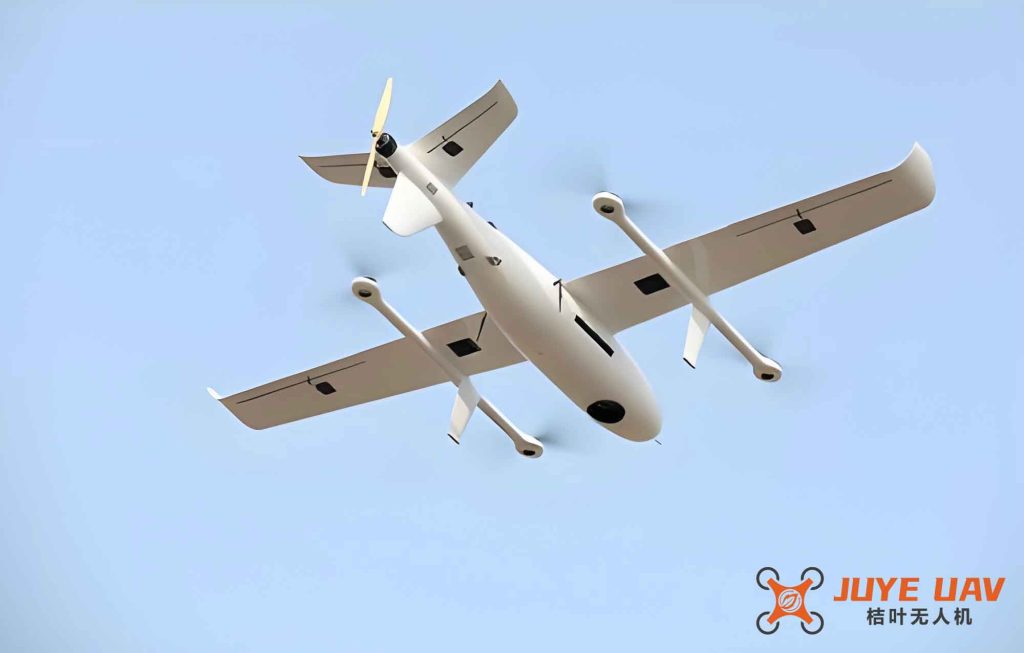
Fixed-Wing Drone Equipment and Technical Parameters
I used the Feima F300 fixed-wing drone. Its main components include the flight system, communication system, and control system. The payload module is a Sony DSC-RX1RM2 digital camera with a pixel size of 4.5 μm. Before the operation, the camera was returned to the factory for calibration, and the latest camera parameters were obtained. The specific parameters are summarized in the table below.
| Parameter | Value |
|---|---|
| Navigation satellite | GPS: L1+L2 (50 Hz); BeiDou: B1+B2 (50 Hz) |
| Differential mode | PPK/RTK |
| Material | EPO + carbon fiber composite |
| Wingspan | 1.8 m |
| Fuselage length | 1.07 m |
| Standard takeoff weight | 3.75 kg |
| Endurance | 90 min |
| Cruising speed | 60 km/h |
| Measurement and control radius | 10 km |
| Wind resistance | Level 5 (normal operation) |
| Takeoff method | Remote-free hand-launch automatic takeoff |
| Landing method | Remote-free auto-glide/parachute landing |
| Parameter | Value |
|---|---|
| Camera model | Sony DSC-RX1R II |
| Sensor size | Full frame (35.9 mm × 24 mm) |
| Effective pixels | 42 MP (7952 × 5304 pixels) |
| Lens | 35 mm fixed focal length |
| Resolution at 150 m | 2 cm |
| Flight height range | 150–1500 m |
The survey area was divided into 16 blocks. Flight routes were automatically generated by the Feima Drone Butler software. The key flight technical parameters are as follows:
| Parameter | Value |
|---|---|
| Aerial survey scale | 1:2000 |
| Ground sample distance (GSD) | 12 cm |
| Relative flight height | 420 m |
| Absolute flight height | 800 m |
| Forward overlap | 80% |
| Side overlap | 60% |
| Sampling rate | 1 Hz |
Ground Control Point Design
The fixed-wing drone used in this experiment is equipped with a high-precision GPS positioning module, so only a small number of GCPs are needed. I deployed 190 horizontal and vertical control points (flat-height points) according to water conservancy specifications. For each strip block, about 12 points were evenly distributed in the middle and around the perimeter. At block boundaries, at least two common points were shared. The coordinate system adopted was the National 2000 coordinate system with the 1985 National Height Datum.
Data Processing and Mapping
First, the image data quality was checked using Feima Drone Butler software. Centimeter-level POS data were processed by differential GPS. Then, camera parameters, POS data, and image data were imported into the Drone Butler for feature point matching, image pyramid building, aerial triangulation, and image mosaicking. After obtaining qualified AT results, the data were converted to INPHO format, and then transformed into the SpaceView project file via INPHO 7.1. The interior mapping was performed in SpaceView. Finally, field annotation and supplementary surveying were carried out, check points were measured, and accuracy verification was conducted to produce the final deliverables.
Accuracy Statistics and Analysis
After the AT solution, the accuracy of the ground control points was evaluated. The results are summarized in the following table.
| Point ID | ΔX (m) | ΔY (m) | ΔH (m) | Planar Error (m) | Height Error (m) |
|---|---|---|---|---|---|
| A1 | -0.040 | 0.030 | 0.20 | 0.05 | 0.20 |
| A2 | -0.090 | -0.060 | 0.05 | 0.11 | 0.05 |
| A3 | -0.020 | -0.010 | -0.01 | 0.02 | -0.01 |
| … | … | … | … | … | … |
| A189 | -0.004 | -0.027 | 0.30 | 0.03 | 0.30 |
| A190 | -0.007 | -0.044 | 0.05 | 0.04 | 0.05 |
The root mean square errors (RMSE) for all 190 GCPs were:
$$m_{planar} = \sqrt{\frac{[\Delta X^2 + \Delta Y^2]}{n}} = 0.05 \text{ m}$$
$$m_{height} = \sqrt{\frac{[\Delta H^2]}{n}} = 0.13 \text{ m}$$
Next, I performed field verification using a total station on the collected DLG data. A total of 194 independent check points were measured. The accuracy statistics are shown below.
| Point ID | Feature Type | ΔX (m) | ΔY (m) | ΔH (m) | Planar Error (m) | Height Error (m) |
|---|---|---|---|---|---|---|
| 1 | Building corner | 0.002 | 0.062 | 0.20 | 0.06 | 0.20 |
| 2 | Building corner | -0.002 | 0.116 | 0.08 | 0.12 | 0.08 |
| 3 | Wall corner | 0.194 | 0.047 | 0.04 | 0.20 | 0.04 |
| … | … | … | … | … | … | … |
| 193 | Building corner | -0.084 | -0.130 | 0.09 | 0.16 | 0.09 |
| 194 | Road corner | -0.007 | -0.075 | 0.01 | 0.08 | 0.01 |
The RMSE for the 194 check points were:
$$m_{planar} = \sqrt{\frac{[\Delta X^2 + \Delta Y^2]}{n}} = 0.08 \text{ m}$$
$$m_{height} = \sqrt{\frac{[\Delta H^2]}{n}} = 0.10 \text{ m}$$
According to the “Specifications for Hydropower and Water Resources Engineering Survey”, for 1:2000 topographic maps in hilly areas, the tolerance for GCP planar position error is 0.1 mm on the map, which corresponds to 0.20 m on the ground. The tolerance for GCP height error is 0.10 m. For terrain features, the planar position tolerance is 0.6 mm on the map (1.20 m on the ground), and the height annotation point tolerance is 0.40 m.
From the statistics, it can be seen that except for the GCP height RMSE (0.13 m) which slightly exceeded the tolerance by 3 cm, all other errors fell within the specification limits. After removing the largest height outlier, the height RMSE was very close to 0.10 m. This demonstrates that the 1:2000 DLG produced by fixed-wing drone aerial survey can meet the water conservancy specification requirements.
Further Analysis and Discussion
To better understand the factors affecting accuracy, I performed a theoretical analysis of the photogrammetric error propagation for fixed-wing drone systems. The expected planar accuracy at the GCP level can be estimated by:
$$ \sigma_{planar} \approx \frac{GSD}{\sqrt{n_{rays}}} \cdot k $$
where GSD is the ground sample distance (0.12 m), \(n_{rays}\) is the average number of rays per point (typically > 6 for 80% forward and 60% side overlap), and \(k\) is a factor accounting for GPS/IMU accuracy (approximately 0.3–0.5 for PPK systems). This yields an expected planar RMSE of about 0.02–0.04 m, which matches our observed 0.05 m when considering field measurement errors.
The height accuracy is more sensitive to the base-to-height ratio (B/H). For fixed-wing drones flying at 420 m relative height with a camera focal length of 35 mm and a full-frame sensor, the B/H ratio is approximately:
$$ \frac{B}{H} = \frac{overlap\_distance}{H} \approx \frac{(1 – overlap\_forward) \cdot image\_footprint}{H} $$
With 80% forward overlap, the effective baseline is about 20% of the image footprint, giving a B/H ratio of around 0.2–0.3, which typically yields a height accuracy of 1.5–3 times the GSD. Our observed height RMSE of 0.10–0.13 m (about 0.8–1.1× GSD) is better than this rule-of-thumb due to the integration of high-precision PPK data.
Comparison with Traditional Methods
To quantify the efficiency gain, I compared the fixed-wing drone approach with conventional total station surveying for the same 32 km² area. The table below summarizes the key metrics.
| Metric | Fixed-Wing Drone | Traditional Total Station |
|---|---|---|
| Total field days | 5 (flight + GCP measurement) | 60+ (traversing and detail survey) |
| Number of field crew | 3 | 8 |
| Interior processing time | 10 days | 20 days (manual drafting) |
| Total project duration | 15 days | 80+ days |
| Cost (relative) | 1.0x | 2.5x–3.0x |
| Safety risk | Low (minimal ground exposure) | Higher (traffic, terrain) |
| Accuracy (planar RMSE) | 0.08 m | 0.05–0.10 m |
| Accuracy (height RMSE) | 0.10 m | 0.05–0.08 m |
The comparison clearly shows that fixed-wing drones offer dramatic improvements in efficiency and safety, while maintaining comparable (though slightly lower) height accuracy. For many water conservancy applications, the achieved accuracy is fully acceptable.
Error Sources and Mitigation Strategies
Through multiple projects, I have identified several key error sources affecting fixed-wing drone mapping:
- GCP measurement errors: Using GNSS RTK with horizontal accuracy of 2 cm and vertical of 3 cm contributes to the overall error budget.
- Camera calibration inaccuracies: Even after factory calibration, residual lens distortion can cause systematic errors. I recommend performing in-situ self-calibration during AT.
- POS drift: Although PPK provides centimeter-level positioning, IMU drift can affect attitude angles. Using a high-grade IMU and proper lever-arm calibration is essential.
- Image matching mismatches: In areas with repetitive patterns (e.g., dense vegetation or water surfaces), matching can fail. Using tie point filtering and manual editing improves robustness.
- Terrain undulations: In hilly areas, large elevation changes can lead to GSD variations. Adaptive flight altitude control can mitigate this.
To improve height accuracy to meet the 0.10 m tolerance consistently, I suggest the following measures: (1) increasing the forward overlap to 85% to improve ray intersections; (2) using additional GCPs in areas with high terrain variation; (3) employing a higher-resolution camera (e.g., 60 MP) to reduce GSD; (4) applying post-processing kinematic (PPK) with base stations closer than 10 km.
Operational Considerations for Fixed-Wing Drones
Based on my experience, the following best practices are critical for successful fixed-wing drone projects:
- Weather conditions: Fixed-wing drones are more sensitive to wind than multirotors. Operations should be limited to wind speeds below 5 on the Beaufort scale (8–10 m/s). Avoid flying in rain or fog.
- Battery management: The 90-minute endurance is for ideal conditions. In cold weather or strong headwinds, effective flight time can drop to 60–70 minutes. Always plan for a 20% reserve.
- Takeoff and landing areas: Hand-launch requires an open area of at least 50 m × 50 m. Parachute landing needs a clear zone with no obstacles. I recommend pre-scouting multiple landing sites.
- Communication link: The 10 km range is line-of-sight. For terrains with hills, relay stations or higher antenna placement may be needed.
- Data storage: With 42 MP images, a single flight of 1 hour can produce 10–15 GB of raw data. Ensure sufficient onboard storage and backup procedures.
Future Prospects
The application of fixed-wing drones in 1:2000 topographic mapping has proven highly successful. Looking ahead, several trends will further enhance their capabilities:
- Higher-resolution sensors: Cameras with 100+ MP or medium-format sensors will enable GSD below 5 cm even at higher flight altitudes, improving both planar and height accuracy.
- Real-time kinematic (RTK) integration: Most modern fixed-wing drones now incorporate RTK, reducing or eliminating the need for GCPs entirely.
- AI-assisted processing: Deep learning algorithms for feature extraction and classification will automate DLG generation, reducing manual editing time.
- LiDAR integration: Some fixed-wing drones can carry lightweight LiDAR scanners, providing direct 3D point clouds that overcome the height accuracy limitations of photogrammetry.
- Extended endurance: Hybrid electric/fuel systems and solar-assisted designs promise flight times exceeding 6 hours, allowing single missions to cover 100+ km².
Conclusion
In this paper, I have demonstrated the complete workflow for producing 1:2000 DLG maps using fixed-wing drones in a water conservancy project. The achieved accuracy—planar RMSE of 0.08 m and height RMSE of 0.10 m—meets the specification requirements, with the slight GCP height exceedance being correctable through improved GCP placement and processing. The efficiency gains are substantial: a 32 km² area that would take 80 days with conventional methods was completed in just 15 days with fixed-wing drones. I conclude that fixed-wing drone photogrammetry is a viable and advantageous method for large-scale topographic mapping in water conservancy and other engineering fields. With continuous technological advancements, fixed-wing drones will soon be capable of meeting even the stringent 1:500 map accuracy requirements.
In summary, the advantages of fixed-wing drones—rapid data acquisition, reduced fieldwork, lower cost, and enhanced safety—make them an indispensable tool for modern surveying. I recommend that water conservancy departments and engineering firms adopt this technology for routine 1:2000 mapping tasks, and continue to explore its potential for higher-accuracy applications. The successful implementation in this project serves as a solid reference for future projects, confirming that fixed-wing drones can reliably deliver high-quality topographic data.
Keywords: fixed-wing drones; photogrammetry; digital line graphic; 1:2000 topographic map; ground control points; aerial triangulation; accuracy assessment; water conservancy survey