
In the realm of autonomous systems, reliable navigation is the cornerstone of operational success. For Unmanned Aerial Vehicles (UAVs), this requirement is particularly acute, as they operate in diverse and often unpredictable environments, from dense urban canyons for infrastructure inspection to remote areas for disaster response. A single navigation sensor modality is frequently insufficient. Global Navigation Satellite Systems (GNSS), like GPS, provide absolute positioning but are susceptible to signal blockage, multipath effects, and intentional jamming. Conversely, a Strapdown Inertial Navigation System (SINS) offers continuous, high-frequency, and self-contained motion estimation but suffers from unbounded error growth due to the integration of sensor biases and noise. The fusion of these complementary systems is therefore not just an option but a necessity for achieving the high levels of accuracy, availability, and integrity demanded by modern UAV drone missions. This article presents, from my research perspective, the design and validation of an advanced, tightly coupled GPS/SINS integrated navigation system, engineered to deliver superior performance for UAVs under challenging conditions.
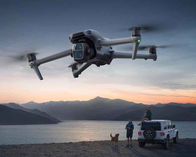
The fundamental challenge for any UAV drone navigation system is to maintain an accurate estimate of its state—position, velocity, and attitude—over time. The SINS algorithm propagates this state using measurements from an Inertial Measurement Unit (IMU), containing triaxial gyroscopes and accelerometers. The core mechanization equations in the navigation frame (n-frame: North-East-Down) are as follows:
Attitude Update (using quaternion q):
$$ \dot{\mathbf{q}}_{b}^{n} = \frac{1}{2} \mathbf{q}_{b}^{n} \otimes \boldsymbol{\omega}_{nb}^{b} $$
where $\boldsymbol{\omega}_{nb}^{b}$ is the angular rate of the body frame (b-frame) relative to the n-frame, expressed in the b-frame, and $\otimes$ denotes quaternion multiplication.
Velocity Update:
$$ \dot{\mathbf{v}}_{eb}^{n} = \mathbf{R}_{b}^{n} \mathbf{f}_{ib}^{b} + \mathbf{g}^{n} – \boldsymbol{\omega}_{en}^{n} \times \mathbf{v}_{eb}^{n} $$
where $\mathbf{R}_{b}^{n}$ is the rotation matrix from b- to n-frame derived from $\mathbf{q}_{b}^{n}$, $\mathbf{f}_{ib}^{b}$ is the specific force measured by accelerometers, $\mathbf{g}^{n}$ is gravity, and $\boldsymbol{\omega}_{en}^{n}$ is the transport rate.
Position Update:
$$ \dot{\mathbf{p}}^{n} = \mathbf{v}_{eb}^{n} $$
where $\mathbf{p}^{n} = [\phi, \lambda, h]^{T}$ represents latitude, longitude, and height.
While these equations provide a continuous solution, even minuscule errors in the IMU measurements—gyro bias $\mathbf{b}_g$ and accelerometer bias $\mathbf{b}_a$—lead to quadratic and cubic error growth in position over time. This is the critical weakness of a stand-alone SINS for a UAV drone on a long-endurance mission.
System Architecture: From Loose to Tight Coupling
To counteract the SINS drift, external aiding from GPS is employed. The integration can be implemented at different levels of sophistication, each with distinct advantages and computational demands. My design emphasizes a tightly coupled architecture as the primary operational mode due to its robustness in signal-degraded environments.
| Coupling Mode | Data Fused in Filter | Advantages | Disadvantages | Suitability for UAV Drone |
|---|---|---|---|---|
| Loose | GPS position & velocity solutions | Simple, low computational cost. | Fails if less than 4 satellites are visible; vulnerable to GPS solution errors. | Open-sky, non-critical missions. |
| Tight | Raw GPS pseudorange (ρ) and pseudorange rate (ṗ) from each satellite. | Works with ≥1 satellite; better mitigates multipath; corrects SINS at a deeper level. | More complex state model; requires GPS receiver data access. | Urban, canyon, or foliage-rich environments (primary mode). |
| Deep/Ultra-tight | SINS info aids GPS tracking loops; raw correlator outputs may be fused. | Superior dynamic tracking and weak-signal performance; highest robustness. | Very high complexity; requires deep integration with receiver hardware. | High-dynamic UAV drones or severe jamming/scintillation conditions. |
The tightly coupled architecture I propose operates on a multi-layer processing principle. The core is an Extended Kalman Filter (EKF) that optimally estimates and corrects the navigation error states. This is supported by a high-fidelity inertial processing chain with advanced compensation and a robust multi-source data fusion layer.
Core Algorithm: The Extended Kalman Filter for State Estimation
The EKF is the optimal estimator for nonlinear systems under the assumption of Gaussian noise. For the UAV drone navigation problem, the system is inherently nonlinear. The EKF linearizes the system around the current best estimate. The process involves two main steps: Prediction (Time Update) and Correction (Measurement Update).
1. State Vector Definition:
The error state vector is chosen for the filter, as it remains small and well-suited for linearization. For a tightly coupled system with clock error estimation, a 17-state vector is common:
$$
\mathbf{x} = [\delta \mathbf{p}^n, \delta \mathbf{v}^n, \boldsymbol{\psi}^n, \delta \mathbf{b}_g, \delta \mathbf{b}_a, \delta b, \delta d]^T
$$
where:
- $\delta \mathbf{p}^n = [\delta \phi, \delta \lambda, \delta h]$: Position errors (lat, lon, height).
- $\delta \mathbf{v}^n = [\delta v_N, \delta v_E, \delta v_D]$: Velocity errors in NED frame.
- $\boldsymbol{\psi}^n = [\psi_N, \psi_E, \psi_D]$: Attitude error angles (misalignment).
- $\delta \mathbf{b}_g, \delta \mathbf{b}_a$: Gyro and accelerometer bias errors.
- $\delta b, \delta d$: GPS receiver clock bias and drift errors (scaled by speed of light c).
2. Prediction Step (SINS Propagation):
The nominal SINS mechanization equations (as above) propagate the full state (position, velocity, attitude, etc.). Simultaneously, the EKF propagates the error state covariance $\mathbf{P}$.
$$
\mathbf{x}_{k|k-1} = \mathbf{\Phi}_k \mathbf{x}_{k-1|k-1}
$$
$$
\mathbf{P}_{k|k-1} = \mathbf{\Phi}_k \mathbf{P}_{k-1|k-1} \mathbf{\Phi}_k^T + \mathbf{Q}_k
$$
Here, $\mathbf{\Phi}_k$ is the state transition matrix, derived by linearizing the SINS error dynamics. $\mathbf{Q}_k$ is the process noise covariance matrix, modeling the intensity of IMU sensor noises (angular random walk, velocity random walk).
3. Measurement Update Step (GPS/Magnetometer Aid):
When GPS measurements are available, they are used to correct the predicted state. In tight coupling, the measurement innovation is the difference between the measured GPS pseudorange/pseudorange rate and the predicted values based on the SINS-estimated position/velocity and the estimated clock states.
Predicted Pseudorange for satellite i:
$$ \hat{\rho}^{(i)} = || \hat{\mathbf{r}}_{ea}^{(i)} – \hat{\mathbf{r}}_{SINS} || + \hat{b} $$
where $\hat{\mathbf{r}}_{ea}^{(i)}$ is the satellite position in ECEF frame, $\hat{\mathbf{r}}_{SINS}$ is the SINS-derived receiver position in ECEF, and $\hat{b}$ is the estimated clock bias.
The linearized measurement model is:
$$ \mathbf{z}_{\rho} = \mathbf{H}_{\rho} \mathbf{x} + \mathbf{v}_{\rho} $$
The design matrix $\mathbf{H}_{\rho}$ for pseudoranges has the following structure for m visible satellites:
$$
\mathbf{H}_{\rho} =
\begin{bmatrix}
\mathbf{H}_{\rho, geo}^{(1)} & \mathbf{0}_{1 \times 9} & \mathbf{0}_{1 \times 3} & 1 & 0\\
\mathbf{H}_{\rho, geo}^{(2)} & \mathbf{0}_{1 \times 9} & \mathbf{0}_{1 \times 3} & 1 & 0\\
\vdots & \vdots & \vdots & \vdots & \vdots\\
\mathbf{H}_{\rho, geo}^{(m)} & \mathbf{0}_{1 \times 9} & \mathbf{0}_{1 \times 3} & 1 & 0
\end{bmatrix}
$$
where $\mathbf{H}_{\rho, geo}^{(i)}$ is the geometric line-of-sight vector from the estimated user position to satellite i, projected into the position error states.
Similarly, for pseudorange rates:
$$ \mathbf{z}_{\dot{\rho}} = \mathbf{H}_{\dot{\rho}} \mathbf{x} + \mathbf{v}_{\dot{\rho}} $$
with $\mathbf{H}_{\dot{\rho}}$ relating to the line-of-sight velocity and clock drift.
Magnetometer Aid: To further control heading drift, especially during GPS outages, a magnetometer providing the magnetic field vector $\mathbf{m}^b$ is integrated. The measurement is the heading angle derived from the horizontal components of the measured field in the navigation frame ($\mathbf{m}^n = \mathbf{R}_b^n \mathbf{m}^b$):
$$ \psi_{mag} = \arctan2(m_E^n, m_N^n) $$
This provides a nonlinear observation of the attitude error, which is linearized within the EKF update sequence.
The standard EKF equations then compute the Kalman gain $\mathbf{K}_k$, update the error state $\mathbf{x}_{k|k}$, and correct the covariance $\mathbf{P}_{k|k}$:
$$
\mathbf{K}_k = \mathbf{P}_{k|k-1} \mathbf{H}_k^T (\mathbf{H}_k \mathbf{P}_{k|k-1} \mathbf{H}_k^T + \mathbf{R}_k)^{-1}
$$
$$
\mathbf{x}_{k|k} = \mathbf{x}_{k|k-1} + \mathbf{K}_k (\mathbf{z}_k – \mathbf{H}_k \mathbf{x}_{k|k-1})
$$
$$
\mathbf{P}_{k|k} = (\mathbf{I} – \mathbf{K}_k \mathbf{H}_k) \mathbf{P}_{k|k-1}
$$
The estimated error state $\mathbf{x}_{k|k}$ is then fed back to correct the SINS nominal states (position, velocity, attitude, biases), completing the closed-loop correction essential for a UAV drone’s long-term stability.
Enhancing Precision: Second-Order Kinematic Compensation
A critical enhancement in the inertial processing chain is the compensation of coning and sculling errors. These are higher-order motion artifacts that arise when the UAV drone undergoes rotational and translational vibrations simultaneously. If ignored, they lead to significant drift in attitude and velocity. Using the incremental angles ($\Delta\boldsymbol{\theta}$) and velocities ($\Delta\mathbf{v}$) over a short IMU sampling period $\Delta t$, the compensated values are:
Coning Correction (for attitude):
$$ \Delta\boldsymbol{\theta}_{corr} = \Delta\boldsymbol{\theta} + \frac{1}{12} (\Delta\boldsymbol{\theta}_{k-1} \times \Delta\boldsymbol{\theta}_k) $$
Sculling Correction (for velocity):
$$ \Delta\mathbf{v}_{corr} = \Delta\mathbf{v} + \frac{1}{2} (\Delta\boldsymbol{\theta} \times \Delta\mathbf{v}) + \frac{1}{6} \Delta\boldsymbol{\theta} \times (\Delta\boldsymbol{\theta} \times \Delta\mathbf{v}) $$
These compensated increments are then used in the precise attitude quaternion update and velocity integration, substantially improving accuracy during dynamic maneuvers typical of a UAV drone flight.
Simulation Analysis and Performance Validation
To validate the performance of the proposed tightly integrated GPS/SINS framework, a comprehensive software simulation was conducted. The simulated UAV drone trajectory included phases of constant velocity, coordinated turns, climbs, and descents, mimicking a realistic urban inspection or search-and-rescue scenario. The sensor error characteristics were modeled as follows:
| Sensor | Parameter | Value / Model |
|---|---|---|
| IMU (SINS) | Gyro Bias Stability | 0.2 °/hr (1σ) |
| Accelerometer Bias | 300 μg (1σ) | |
| Sampling Rate | 50 Hz | |
| GPS Receiver | Horizontal Position Noise | 2.0 m (1σ) |
| Velocity Noise | 0.3 m/s (1σ) | |
| Update Rate | 5 Hz | |
| Magnetometer | Heading Noise | 1.0° (1σ) @ 10 Hz |
The key performance metrics are the Root Mean Square Error (RMSE) and maximum error during the mission. The following table summarizes the navigation performance of the proposed Tightly Coupled EKF (TC-EKF) system against a stand-alone SINS and a traditional Loosely Coupled EKF (LC-EKF) during a simulated 600-second flight, which included a 60-second GPS signal outage to test robustness.
| Navigation System | Horizontal Position RMSE (m) | Vertical Position RMSE (m) | Velocity RMSE (m/s) | Max Horizontal Error During Outage (m) |
|---|---|---|---|---|
| Stand-alone SINS | > 500 (diverged) | > 200 (diverged) | > 10 (diverged) | N/A (unbounded) |
| LC-EKF | 2.5 | 3.8 | 0.35 | 25.1 (grows rapidly) |
| Proposed TC-EKF | 1.8 | 2.2 | 0.25 | 8.7 (well-bounded) |
The results are clear. The tightly coupled system demonstrates a ~30% improvement in horizontal positioning accuracy (1.8 m RMSE vs. 2.5 m) over the loose coupling approach under nominal GPS conditions. More importantly, during the simulated GPS denial period, the error growth of the TC-EKF system was dramatically lower. The maximum horizontal error was contained below 9 meters, compared to over 25 meters for the LC-EKF. This is primarily due to two factors inherent to the tight coupling design: 1) the continued use of any available satellite signals (even if less than four) during partial outages, which provides some geometric constraint, and 2) the more accurate and direct estimation of IMU sensor biases (δb_g, δb_a) using the raw GPS measurements, leading to a better-calibrated SINS during the outage. This robust performance is exactly what is required for a UAV drone navigating near buildings or under tree canopies where short GPS dropouts are frequent.
The estimator’s performance in tracking critical sensor errors is also noteworthy. The following plot conceptually illustrates the EKF’s estimation of the gyroscope biases. The X and Y axis biases (aligned with the UAV drone’s roll and pitch axes) are effectively observed and corrected through the combination of GPS velocity updates and the magnetometer’s heading aid. The Z-axis (yaw) bias, which is particularly challenging for a pure SINS, is directly constrained by the magnetometer updates, keeping its estimated value within a very tight bound (e.g., ±0.25 x 10^-3 °/s), as predicted by the observability analysis of the system. This effective bias estimation is the key to the system’s long-term stability.
Conclusion and Future Directions for UAV Drone Navigation
The integration of GPS and SINS via a tightly coupled Extended Kalman Filter framework, augmented with second-order kinematic compensation and multi-source data fusion (including magnetometers), presents a powerful solution for high-performance UAV drone navigation. This architecture directly addresses the core limitations of each subsystem: it mitigates the long-term drift of the SINS by frequent GPS corrections at the raw measurement level, and it preserves navigation capability during partial or intermittent GPS signal degradation by leveraging the well-calibrated inertial system. The simulation results confirm significant gains in both accuracy and, crucially, robustness, making it suitable for demanding applications like autonomous urban inspection, precision agriculture, and disaster area mapping.
Future work will focus on further enhancing this framework. The incorporation of additional aiding sources is a logical next step. Visual odometry or LiDAR-based SLAM (Simultaneous Localization and Mapping) could provide precise relative motion updates in GPS-denied environments, seamlessly integrating into the EKF’s measurement update sequence. Furthermore, exploring more advanced nonlinear filtering techniques, such as the Unscented Kalman Filter (UKF) or Particle Filters, may offer benefits during extreme dynamic maneuvers where the EKF’s linearization assumptions are strained. Finally, implementing and testing this algorithm on real UAV drone hardware with commercial-grade MEMS-IMUs and GPS receivers will be essential to validate its practical performance and computational efficiency in the field, paving the way for its adoption in next-generation autonomous aerial systems.