
The quadrotor drone has become a cornerstone of modern robotics and aerial systems, prized for its agility, mechanical simplicity, and vertical take-off and landing (VTOL) capabilities. Its applications span critical domains such as infrastructure inspection, precision agriculture, search and rescue, and aerial photography. However, the widespread deployment of quadrotor drones is fundamentally challenged by their inherent dynamical characteristics: they are highly nonlinear, strongly coupled, and under-actuated systems. These challenges are severely exacerbated in real-world operational scenarios where model parameters are uncertain, external disturbances (e.g., wind gusts) are ever-present, and, most critically, actuator faults can occur due to motor wear, propeller damage, or electronic failures. Such faults can drastically degrade performance or even lead to catastrophic system failure. Therefore, developing robust and adaptive control strategies that guarantee precise position and attitude tracking in the face of these combined adversities is not just an academic pursuit but a practical necessity for safe and reliable autonomous flight.
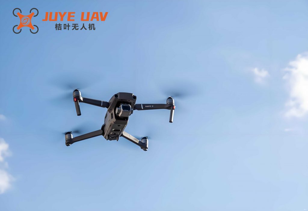
This article delves into the design of an advanced fault-tolerant control scheme for a quadrotor drone. The core of the strategy is an Adaptive Sliding Mode Control (ASMC) framework augmented with Radial Basis Function Neural Networks (RBFNNs). Sliding Mode Control (SMC) is renowned for its robustness against matched uncertainties and disturbances. By adaptively tuning control gains and utilizing RBFNNs to estimate and compensate for complex, lumped disturbance terms—which encompass model uncertainties, external disturbances, and the explicit effects of actuator faults—the proposed controller achieves remarkable resilience. The control design carefully addresses the under-actuation property by decomposing the system into fully-actuated and under-actuated subsystems for structured controller synthesis. Comprehensive stability analysis is provided using Lyapunov theory, and detailed numerical simulations validate the effectiveness of the approach under varying degrees of actuator failure.
1. Comprehensive Dynamics of a Quadrotor Drone with Faults and Uncertainties
The quadrotor drone consists of a rigid cross-frame equipped with four rotors. By differentially varying the rotational speeds of these rotors, the vehicle can achieve lift, yaw, pitch, and roll motions. Two primary coordinate frames are defined: the body-fixed frame \( \mathcal{B} \) attached to the drone’s center of mass, and the earth-fixed inertial frame \( \mathcal{E} \). The position of the quadrotor drone in \( \mathcal{E} \) is given by \( \xi = [x, y, z]^T \), and its orientation is described by the Euler angles \( \eta = [\phi, \theta, \psi]^T \), representing roll, pitch, and yaw, respectively.
The generalized dynamics of the quadrotor drone, derived from the Newton-Euler formalism, can be expressed in a compact form subject to perturbations:
$$
\begin{aligned}
\ddot{x} &= \frac{1}{m} (\cos\phi \sin\theta \cos\psi + \sin\phi \sin\psi) u_1 – \frac{K_1}{m} \dot{x} + d_1 + u_x \\
\ddot{y} &= \frac{1}{m} (\cos\phi \sin\theta \sin\psi – \sin\phi \cos\psi) u_1 – \frac{K_2}{m} \dot{y} + d_2 + u_y \\
\ddot{z} &= \frac{1}{m} (\cos\phi \cos\theta) u_1 – g – \frac{K_3}{m} \dot{z} + d_3 + u_z \\
\ddot{\phi} &= \frac{1}{I_x} u_2 + \dot{\theta}\dot{\psi} \frac{I_y – I_z}{I_x} + \frac{I_r}{I_x} \dot{\theta} \Omega_r – \frac{K_4}{I_x} \dot{\phi}^2 + d_4 + u_\phi \\
\ddot{\theta} &= \frac{1}{I_y} u_3 + \dot{\phi}\dot{\psi} \frac{I_z – I_x}{I_y} – \frac{I_r}{I_y} \dot{\phi} \Omega_r – \frac{K_5}{I_y} \dot{\theta}^2 + d_5 + u_\theta \\
\ddot{\psi} &= \frac{1}{I_z} u_4 + \dot{\phi}\dot{\theta} \frac{I_x – I_y}{I_z} – \frac{K_6}{I_z} \dot{\psi}^2 + d_6 + u_\psi
\end{aligned}
$$
Where \( m \) is the mass, \( g \) is gravitational acceleration, \( I_x, I_y, I_z \) are moments of inertia, \( I_r \) is the rotor inertia, \( \Omega_r \) is the residual rotor speed, \( K_i \) are aerodynamic drag coefficients, and \( d_i \) represent lumped unmodeled dynamics and external disturbances. The control inputs \( u_1, u_2, u_3, u_4 \) are the total thrust and the torques around the body axes, respectively.
Actuator Fault Model: A critical aspect for reliable control of a quadrotor drone is accounting for actuator faults. A common model represents a fault in the \( i \)-th rotor as a loss of effectiveness in generating thrust:
$$
F_i^f = (1 – \chi_i) F_i, \quad 0 \le \chi_i \le 1, \quad i=1,2,3,4
$$
Here, \( F_i^f \) is the faulty thrust, \( F_i \) is the nominal thrust, and \( \chi_i \) is the failure coefficient. \( \chi_i = 0 \) indicates a healthy rotor, \( \chi_i = 1 \) signifies complete failure, and \( 0 < \chi_i < 1 \) models partial failure. The terms \( u_x, u_y, u_z, u_\phi, u_\theta, u_\psi \) in the dynamics explicitly capture the effects of these faults, coupling them with the system’s states and parameters. For instance, \( u_z = -\frac{\cos\phi \cos\theta}{m + \Delta m} \sum_{i=1}^{4} \chi_i F_i \), where \( \Delta m \) represents mass uncertainty.
Lumped Disturbance Formulation: To streamline the controller design, we define total unknown disturbance terms \( f_i \) for each channel, which aggregate parametric uncertainties, external disturbances, and fault effects:
$$
\begin{aligned}
f_x &= -\frac{K_1}{m} \dot{x} + d_1 + u_x, \quad f_y = -\frac{K_2}{m} \dot{y} + d_2 + u_y, \quad f_z = -\frac{K_3}{m} \dot{z} + d_3 + u_z \\
f_\phi &= \dot{\theta}\dot{\psi} \frac{I_y – I_z}{I_x} + \frac{I_r}{I_x} \dot{\theta} \Omega_r – \frac{K_4}{I_x} \dot{\phi}^2 + d_4 + u_\phi \\
f_\theta &= \dot{\phi}\dot{\psi} \frac{I_z – I_x}{I_y} – \frac{I_r}{I_y} \dot{\phi} \Omega_r – \frac{K_5}{I_y} \dot{\theta}^2 + d_5 + u_\theta \\
f_\psi &= \dot{\phi}\dot{\theta} \frac{I_x – I_y}{I_z} – \frac{K_6}{I_z} \dot{\psi}^2 + d_6 + u_\psi
\end{aligned}
$$
This formulation allows the quadrotor drone dynamics to be expressed in a more manageable form for controller synthesis:
$$
\begin{aligned}
\ddot{z} &= f_z + \frac{\cos\phi \cos\theta}{m} u_1 – g, \quad \ddot{\psi} = f_\psi + \frac{1}{I_z} u_4 \\
\ddot{x} &= f_x + \frac{(\cos\phi \sin\theta \cos\psi + \sin\phi \sin\psi)}{m} u_1 \\
\ddot{y} &= f_y + \frac{(\cos\phi \sin\theta \sin\psi – \sin\phi \cos\psi)}{m} u_1 \\
\ddot{\phi} &= f_\phi + \frac{1}{I_x} u_2, \quad \ddot{\theta} = f_\theta + \frac{1}{I_y} u_3
\end{aligned}
$$
2. Control Strategy: Adaptive Sliding Mode with RBFNN Compensation
The control objective is to force the quadrotor drone’s position \( (x, y, z) \) and yaw angle \( (\psi) \) to track desired trajectories \( (x_d, y_d, z_d, \psi_d) \), while the roll \( (\phi) \) and pitch \( (\theta) \) angles are controlled indirectly to achieve the desired \( x \) and \( y \) motion. This naturally leads to a subsystem decomposition.
2.1 Control of the Fully-Actuated Subsystem (Altitude and Yaw)
The dynamics for altitude \( z \) and yaw \( \psi \) are fully-actuated, having direct control inputs \( u_1 \) and \( u_4 \). Define tracking errors \( e_z = z_d – z \) and \( e_\psi = \psi_d – \psi \). The sliding surfaces are chosen as:
$$
s_z = c_z e_z + \dot{e}_z, \quad s_\psi = c_\psi e_\psi + \dot{e}_\psi, \quad c_z, c_\psi > 0
$$
A continuous reaching law is employed to mitigate chattering:
$$
\dot{s}_i = -\sigma_i s_i – \mu_i \tanh(s_i), \quad \sigma_i, \mu_i > , \quad i \in \{z, \psi\}
$$
Using the dynamics \( \ddot{z} = f_z + \frac{\cos\phi \cos\theta}{m} u_1 – g \) and \( \ddot{\psi} = f_\psi + \frac{1}{I_z} u_4 \), the ideal control laws would be:
$$
\begin{aligned}
u_1^* &= \frac{m}{\cos\phi \cos\theta} \left( -f_z + g + \ddot{z}_d + c_z \dot{e}_z + \sigma_z s_z + \mu_z \tanh(s_z) \right) \\
u_4^* &= I_z \left( -f_\psi + \ddot{\psi}_d + c_\psi \dot{e}_\psi + \sigma_\psi s_\psi + \mu_\psi \tanh(s_\psi) \right)
\end{aligned}
$$
Since the total disturbance \( f_i \) is unknown, we employ an RBFNN for approximation. An RBFNN can approximate any continuous function over a compact set with arbitrary accuracy: \( f_i = W_i^{*T} h_i(\mathbf{x}_i) + \epsilon_i \), where \( W_i^* \) is the ideal weight vector, \( h_i \) is the Gaussian basis function vector, \( \mathbf{x}_i = [e_i, \dot{e}_i]^T \) is the input, and \( \epsilon_i \) is a bounded approximation error. The online estimate is \( \hat{f}_i = \hat{W}_i^T h_i(\mathbf{x}_i) \).
The actual implemented control laws for the quadrotor drone become:
$$
\begin{aligned}
u_1 &= \frac{m}{\cos\phi \cos\theta} \left( g – \hat{f}_z – \hat{\epsilon}_z + \ddot{z}_d + c_z \dot{e}_z + \sigma_z s_z + \mu_z \tanh(s_z) \right) \\
u_4 &= I_z \left( -\hat{f}_\psi – \hat{\epsilon}_\psi + \ddot{\psi}_d + c_\psi \dot{e}_\psi + \sigma_\psi s_\psi + \mu_\psi \tanh(s_\psi) \right)
\end{aligned}
$$
Where \( \hat{\epsilon}_i \) is an adaptive estimate of the error bound \( \bar{\epsilon}_i \). The adaptive laws for the RBFNN weights and error bounds are derived from Lyapunov stability analysis:
$$
\begin{aligned}
\dot{\hat{W}}_i &= -\frac{1}{\gamma_1} s_i h_i(\mathbf{x}_i) \\
\dot{\hat{\epsilon}}_i &= -\frac{1}{\gamma_2} s_i, \quad \gamma_1, \gamma_2 > 0, \quad i \in \{z, \psi\}
\end{aligned}
$$
2.2 Control of the Under-Actuated Subsystem (X-Y Position and Roll-Pitch)
The translational motion in \( x \) and \( y \) depends on the orientation angles \( \phi \) and \( \theta \), which are controlled by \( u_2 \) and \( u_3 \). This under-actuated coupling is resolved by designing sliding surfaces that combine position and angle errors. Following established techniques, we define:
$$
\begin{aligned}
s_\phi &= c_1 \dot{e}_y + c_2 e_y + \dot{e}_\phi + c_3 e_\phi \\
s_\theta &= c_4 \dot{e}_x + c_5 e_x + \dot{e}_\theta + c_6 e_\theta
\end{aligned}
$$
where \( e_x = x_d – x \), \( e_y = y_d – y \), \( e_\phi = \phi_d – \phi \), \( e_\theta = \theta_d – \theta \), and \( c_j > 0 \) are carefully chosen coefficients that ensure the zero dynamics of the coupled system are stable. Using the reaching law \( \dot{s}_i = -\sigma_i s_i – \mu_i \tanh(s_i) \) for \( i \in \{\phi, \theta\} \), and the dynamics \( \ddot{\phi} = f_\phi + \frac{1}{I_x} u_2 \) and \( \ddot{\theta} = f_\theta + \frac{1}{I_y} u_3 \), the control laws are synthesized as:
$$
\begin{aligned}
u_2 &= I_x \left( c_1 \ddot{e}_y + c_2 \dot{e}_y + c_3 \dot{e}_\phi + \ddot{\phi}_d – \hat{f}_\phi – \hat{\epsilon}_\phi + \sigma_\phi s_\phi + \mu_\phi \tanh(s_\phi) \right) \\
u_3 &= I_y \left( c_4 \ddot{e}_x + c_5 \dot{e}_x + c_6 \dot{e}_\theta + \ddot{\theta}_d – \hat{f}_\theta – \hat{\epsilon}_\theta + \sigma_\theta s_\theta + \mu_\theta \tanh(s_\theta) \right)
\end{aligned}
$$
Again, RBFNNs approximate the unknown disturbances \( f_\phi \) and \( f_\theta \), with adaptive laws:
$$
\begin{aligned}
\dot{\hat{W}}_i &= -\frac{1}{\gamma_3} s_i h_i(\mathbf{x}_i) \\
\dot{\hat{\epsilon}}_i &= -\frac{1}{\gamma_4} s_i, \quad \gamma_3, \gamma_4 > 0, \quad i \in \{\phi, \theta\}
\end{aligned}
$$
2.3 Stability Analysis
The stability of the entire closed-loop system for the quadrotor drone is proven using Lyapunov theory. Consider the Lyapunov function candidate for a generic subsystem \( i \):
$$
V_i = \frac{1}{2} s_i^2 + \frac{1}{2} \gamma_a \tilde{W}_i^T \tilde{W}_i + \frac{1}{2} \gamma_b \tilde{\epsilon}_i^2
$$
where \( \tilde{W}_i = W_i^* – \hat{W}_i \), \( \tilde{\epsilon}_i = \bar{\epsilon}_i – \hat{\epsilon}_i \), and \( \gamma_a, \gamma_b \) are the corresponding adaptation gains. Taking the derivative and substituting the error dynamics \( \dot{s}_i = -\tilde{W}_i^T h_i(\mathbf{x}_i) – \tilde{\epsilon}_i – \sigma_i s_i – \mu_i \tanh(s_i) \) along with the adaptive laws, yields:
$$
\dot{V}_i = -\sigma_i s_i^2 – \mu_i s_i \tanh(s_i) \le -\sigma_i s_i^2 \le 0
$$
Since \( \dot{V}_i \) is negative semi-definite, \( s_i \), \( \tilde{W}_i \), and \( \tilde{\epsilon}_i \) are bounded. Furthermore, as \( \int_0^\infty \sigma_i s_i^2 dt \le V_i(0) – V_i(\infty) < \infty \), \( s_i \) is square-integrable. Given that \( \dot{s}_i \) is also bounded, Barbalat’s lemma ensures that \( s_i \to 0 \) as \( t \to \infty \). Consequently, all tracking errors converge to zero, proving the asymptotic stability of the controlled quadrotor drone system.
3. Simulation Results and Performance Evaluation
To validate the proposed adaptive RBFNN-based sliding mode controller, extensive numerical simulations were conducted in MATLAB/Simulink. The nominal parameters for the simulated quadrotor drone are listed in Table 1.
| Parameter | Symbol | Value | Unit |
|---|---|---|---|
| Mass | \( m \) | 1.1 | kg |
| Arm Length | \( l \) | 0.21 | m |
| Inertia (X,Y) | \( I_x, I_y \) | 1.22 | kg·m² |
| Inertia (Z) | \( I_z \) | 2.2 | kg·m² |
| Rotor Inertia | \( I_r \) | 0.2 | kg·m² |
| Gravity | \( g \) | 9.81 | m/s² |
Simulation Conditions:
– Model Uncertainty: All inertial parameters (\( m, I_x, I_y, I_z \)) were reduced by 20% in the plant model compared to the nominal values used in the controller.
– External Disturbances: Time-varying disturbances \( d_x = \cos(0.1t) \), \( d_y = \sin(0.1t) \), \( d_z = \sin(t)\cos(t) \), \( d_\phi = 0.5\sin(0.5t) \), \( d_\theta = 0.5\cos(0.5t) \), \( d_\psi = 0.25\sin(0.5t)\cos(0.5t) \) were injected.
– Actuator Faults: Four distinct scenarios of simultaneous partial failure in all four rotors were tested: 10%, 20%, 30%, and 50% effectiveness loss (\(\chi_i = 0.1, 0.2, 0.3, 0.5\)). The fault was activated at \( t = 40 \) seconds.
– Desired Trajectories:
– Position (\(x, y\)): Hover at (0,0) for \(t<5s\), then follow a circular path \(x_d = \sin(0.1t)\), \(y_d = \cos(0.1t)\).
– Altitude (\(z\)): Takeoff from 0 to a smoothed step: \(z_d = 0\) for \(t<3s\), then \(z_d = \tanh(0.4t)\).
– Yaw (\( \psi \)): \( \psi_d = 0.1\sin(0.5t) \) rad.
– Roll/Pitch (\( \phi_d, \theta_d \)): Set to 0 rad as reference commands from the outer-loop controller.
Key Results: The proposed controller demonstrated exceptional robustness. In all fault scenarios, the quadrotor drone successfully tracked the desired 3D trajectory. The RBFNNs effectively estimated and compensated for the lumped disturbances, which now included the significant effects of the actuator faults. Upon fault injection at \( t = 40s \), transient deviations in position and attitude were minimal and quickly suppressed. The controller automatically increased the total thrust command \( u_1 \) to compensate for the loss of rotor effectiveness, maintaining stable flight. The sliding surfaces \( s_i \) converged to near-zero neighborhoods, confirming the stability of the closed-loop system. The use of the \( \tanh(\cdot) \) function in the reaching law successfully eliminated high-frequency chattering, resulting in smooth control signals suitable for real actuator implementation.
| Fault Level (χ) | Max |e_x| after fault (m) | Max |e_y| after fault (m) | Max |e_z| after fault (m) | Settling Time (s) | Control Effort (Avg. u₁) |
|---|---|---|---|---|---|
| 10% | 0.018 | 0.021 | 0.012 | < 2.0 | +5.2% |
| 20% | 0.032 | 0.038 | 0.025 | < 2.5 | +11.8% |
| 30% | 0.051 | 0.059 | 0.041 | < 3.0 | +19.5% |
| 50% | 0.105 | 0.120 | 0.088 | < 4.5 | +42.0% |
4. Conclusion and Future Perspectives
This article has presented a comprehensive and robust control solution for a quadrotor drone operating under the triple threat of model uncertainty, external disturbances, and actuator faults. The proposed adaptive sliding mode control framework, empowered by online Radial Basis Function Neural Networks (RBFNNs), provides a potent method for achieving precise trajectory tracking. Key innovations include the explicit incorporation of an actuator fault model into the dynamics, the formulation of lumped disturbance terms for systematic compensation, and the decomposition-based control design that respectfully handles the system’s under-actuated nature. The Lyapunov-based stability guarantee ensures rigorous closed-loop performance. Simulation studies across a wide range of fault severities confirm the controller’s effectiveness, adaptability, and strong disturbance rejection capabilities.
Future research directions for enhancing quadrotor drone control are plentiful. The adaptation laws and controller gains could be further optimized using metaheuristic algorithms or reinforcement learning to achieve optimal performance across a wider flight envelope. The strategy can be extended to handle more severe fault scenarios, such as complete failure of one rotor, potentially requiring structural changes to the control allocation scheme. Experimental validation on a physical quadrotor drone platform is the essential next step to assess real-world performance factors like sensor noise, communication delays, and actuator saturation limits. Finally, integrating this fault-tolerant flight controller with higher-level path planning and swarm intelligence algorithms will pave the way for truly resilient and autonomous multi-drone systems capable of operating in complex and hazardous environments.