
The rapid advancement and widespread deployment of unmanned aerial vehicles (UAVs), particularly quadrotor drones, have revolutionized numerous fields including aerial photography, surveillance, logistics, and environmental monitoring. Their appeal lies in their mechanical simplicity, agility, vertical take-off and landing capability, and relatively low cost. However, the reliable and safe operation of these systems, especially in the presence of component faults, remains a critical challenge. Among various potential failures, actuator faults—such as motor degradation, propeller damage, or partial loss of effectiveness—are particularly hazardous as they can directly lead to a catastrophic loss of stability and control. Therefore, developing advanced control strategies that can tolerate such faults while maintaining desirable flight performance is of paramount importance for the practical deployment of quadrotor drones.
Traditional control approaches often assume fully functional actuators. When a fault occurs, these controllers may fail to stabilize the system. Fault-Tolerant Control (FTC) schemes are designed to address this issue. Adaptive control has emerged as a powerful tool within FTC, enabling the controller to adjust its parameters online to compensate for unknown faults and uncertainties without requiring an exact fault diagnosis. Meanwhile, ensuring that the closed-loop system not only remains stable but also exhibits prescribed transient and steady-state performance—such as maximum overshoot, convergence rate, and steady-state error bounds—is crucial for practical applications. The concept of Prescribed Performance Control (PPC) provides an elegant framework to enforce such behavioral constraints on the tracking error.
In this article, I present a comprehensive adaptive control scheme integrated with a prescribed performance framework for a quadrotor drone subject to unknown actuator faults. The core contributions of this work are: 1) the development of a dual-loop control structure that decouples the underactuated dynamics into separate translational and rotational subsystems; 2) the design of adaptive laws to estimate and compensate for unknown actuator fault parameters (both loss of effectiveness and additive bias) in real-time; and 3) the incorporation of a prescribed performance function to guarantee that the tracking errors evolve within a designer-specified performance envelope, ensuring predictable and satisfactory system behavior despite the occurrence of faults.
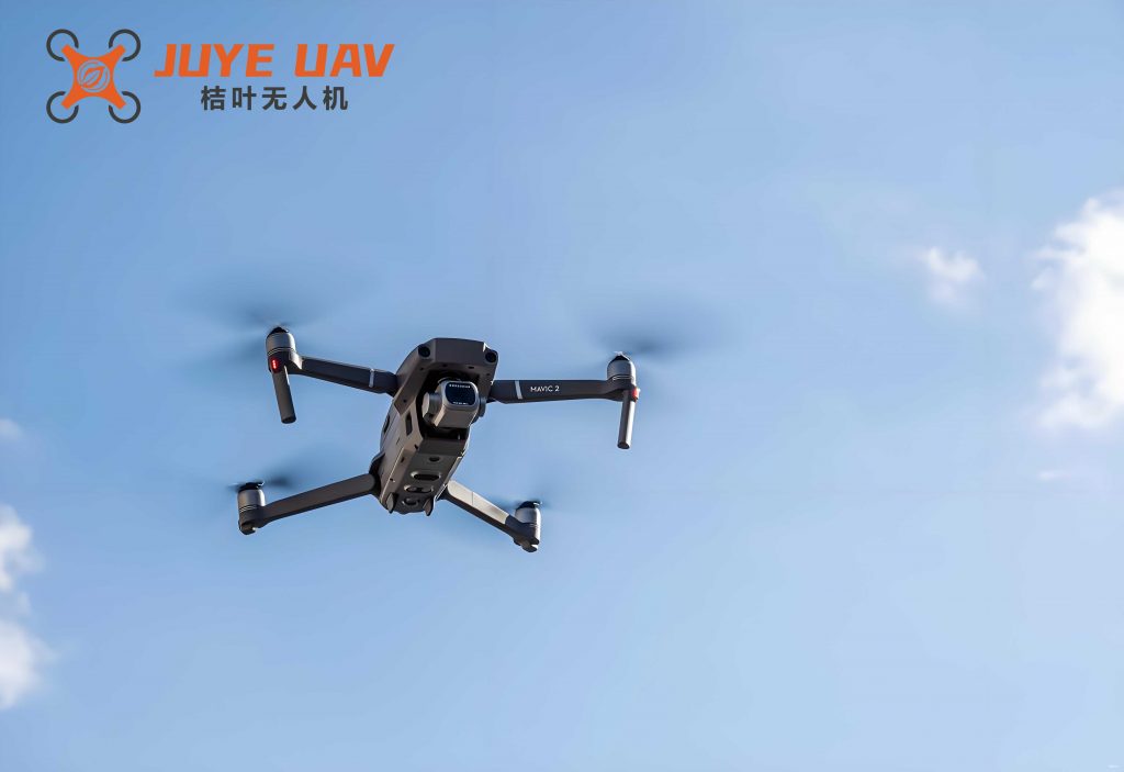
Dynamical Model of a Quadrotor Drone
The standard dynamical model of a quadrotor drone is derived under the assumptions of a rigid and symmetrical structure, with the center of gravity coinciding with the geometric center. Two coordinate frames are defined: the inertial frame \(\{O_e, X_e, Y_e, Z_e\}\) and the body-fixed frame \(\{O_b, X_b, Y_b, Z_b\}\). The position of the vehicle’s center of mass in the inertial frame is denoted by \((x, y, z)\), and its orientation is described by the Euler angles \((\phi, \theta, \psi)\) representing roll, pitch, and yaw, respectively. The control inputs are the total thrust \(u_z\) and the torques \(u_\phi\), \(u_\theta\), \(u_\psi\). The simplified nonlinear dynamics are given by:
$$
\begin{aligned}
\ddot{x} &= \frac{1}{m} (\cos\phi \sin\theta \cos\psi + \sin\phi \sin\psi) u_z, \\
\ddot{y} &= \frac{1}{m} (\cos\phi \sin\theta \sin\psi – \sin\phi \cos\psi) u_z, \\
\ddot{z} &= -\frac{\cos\phi \cos\theta}{m} u_z + g, \\
\ddot{\phi} &= \dot{\theta}\dot{\psi} \frac{I_{yy} – I_{zz}}{I_{xx}} + \dot{\theta} \frac{J_P}{I_{xx}} \Omega_r + \frac{l}{I_{xx}} u_\phi, \\
\ddot{\theta} &= \dot{\phi}\dot{\psi} \frac{I_{zz} – I_{xx}}{I_{yy}} + \dot{\phi} \frac{J_P}{I_{yy}} \Omega_r + \frac{l}{I_{yy}} u_\theta, \\
\ddot{\psi} &= \dot{\phi}\dot{\theta} \frac{I_{xx} – I_{yy}}{I_{zz}} + \frac{l}{I_{zz}} u_\psi.
\end{aligned}
$$
Where \(m\) is the mass, \(g\) is gravitational acceleration, \(l\) is the arm length, \(I_{xx}, I_{yy}, I_{zz}\) are moments of inertia, \(J_P\) is the propeller’s moment of inertia, and \(\Omega_r = -\Omega_1 + \Omega_2 – \Omega_3 + \Omega_4\) is the residual rotor speed. For controller design, the system is often decoupled into an outer position loop and an inner attitude loop.
Actuator Fault Model
Actuator faults in a quadrotor drone can arise from motor wear, electronic speed controller (ESC) malfunctions, or propeller damage. A comprehensive model capturing both loss of effectiveness and additive faults for the \(i\)-th actuator (\(i \in \{z, \phi, \theta, \psi\}\)) is:
$$
u_i = \tau_i u_{i_a} + u_{i_f}.
$$
Here, \(u_i\) is the actual output of the faulty actuator, \(u_{i_a}\) is the controller’s designed command, \(0 \le \tau_i \le 1\) is an unknown effectiveness factor, and \(u_{i_f}\) is an unknown constant additive fault. This model encapsulates several common fault types, as summarized below:
| Fault Type | Condition on \(\tau_i\) | Condition on \(u_{i_f}\) |
|---|---|---|
| Healthy | \(\tau_i = 1\) | \(u_{i_f} = 0\) |
| Partial Loss of Effectiveness | \(0 < \tau_i < 1\) | \(u_{i_f} = 0\) |
| Bias Fault | \(\tau_i = 1\) | \(u_{i_f} \neq 0\) |
| Stuck (Lock-in-Place) | \(\tau_i = 0\) | \(u_{i_f} \neq 0\) |
The control objective is to design \(u_{i_a}\) such that the quadrotor drone tracks a desired trajectory \((x_d, y_d, z_d, \psi_d)\) while compensating for the unknown parameters \(\tau_i\) and \(u_{i_f}\), and ensuring prescribed performance of the tracking errors.
Control Strategy and Prescribed Performance Framework
Dual-Loop Control Structure
I employ a cascaded control structure. The outer loop controls the translational \((x, y, z)\) dynamics and generates desired roll (\(\phi_d\)) and pitch (\(\theta_d\)) angles. The inner loop controls the rotational \((\phi, \theta, \psi)\) dynamics to track these desired angles swiftly. This structure effectively handles the underactuation of the quadrotor drone.
Prescribed Performance and Error Transformation
To enforce predefined transient and steady-state performance on a tracking error \(z_{i1}(t)\) (e.g., \(z_{x1} = x – x_d\)), I constrain it to evolve within a decaying envelope:
$$
-\delta_i \mu_i(t) < z_{i1}(t) < \bar{\delta}_i \mu_i(t), \quad \forall t \ge 0.
$$
The performance function \(\mu_i(t)\) is chosen as a smooth, exponentially decaying function:
$$
\mu_i(t) = (\mu_{i0} – \mu_{i\infty}) e^{-\gamma_i t} + \mu_{i\infty},
$$
where \(\mu_{i0} > \mu_{i\infty} > 0\), \(\gamma_i > 0\), and \(\delta_i, \bar{\delta}_i\) are positive constants defining the relative bounds. The function \(\mu_i(t)\) dictates the maximum allowable overshoot (\(\mu_{i0}\)), the convergence rate (\(\gamma_i\)), and the ultimate bound (\(\mu_{i\infty}\)). To transform this constrained problem into an unconstrained one, I define a smooth, strictly increasing function \(S(\varepsilon_i)\):
$$
z_{i1}(t) = \mu_i(t) S(\varepsilon_i), \quad S(\varepsilon_i) = \frac{\bar{\delta}_i e^{\varepsilon_i} – \delta_i e^{-\varepsilon_i}}{e^{\varepsilon_i} + e^{-\varepsilon_i}}.
$$
The inverse transformation is:
$$
\varepsilon_i = S^{-1}\left( \frac{z_{i1}}{\mu_i} \right) = \frac{1}{2} \ln \left( \frac{\frac{z_{i1}}{\mu_i} + \delta_i}{\bar{\delta}_i – \frac{z_{i1}}{\mu_i}} \right).
$$
The stability of the transformed error \(\varepsilon_i\) now directly implies that the original error \(z_{i1}\) satisfies the prescribed performance bounds. The derivative \(\dot{\varepsilon}_i\) is:
$$
\dot{\varepsilon}_i = r_i \left( \dot{z}_{i1} – \frac{z_{i1}\dot{\mu}_i}{\mu_i} \right), \quad \text{where} \quad r_i = \frac{1}{2\mu_i} \left( \frac{1}{\frac{z_{i1}}{\mu_i} + \delta_i} – \frac{1}{\bar{\delta}_i – \frac{z_{i1}}{\mu_i}} \right) > 0.
$$
This transformation is applied to all tracking errors in both the position and attitude loops of the quadrotor drone.
Adaptive Prescribed Performance Controller Design
The state vector is defined as \(\mathbf{x} = [x_1, …, x_{12}]^T = [x, \dot{x}, y, \dot{y}, z, \dot{z}, \phi, \dot{\phi}, \theta, \dot{\theta}, \psi, \dot{\psi}]^T\). The design proceeds subsystem by subsystem. I will illustrate the detailed design for the altitude (\(z\)) and roll (\(\phi\)) subsystems; the others follow a similar procedure.
Altitude (\(z\)) Subsystem Control
The altitude dynamics from the model are:
$$
\begin{aligned}
\dot{x}_5 &= x_6, \\
\dot{x}_6 &= a_z + b_z u_z, \quad \text{with} \quad a_z = g, \quad b_z = -\frac{\cos x_7 \cos x_9}{m}.
\end{aligned}
$$
Define the tracking error and its derivative: \(z_{z1} = x_5 – z_d\), \(z_{z2} = x_6 – \alpha_z\), where \(\alpha_z\) is a virtual control law. Applying the PPC transformation to \(z_{z1}\) yields the transformed error \(\varepsilon_z\).
Step 1: Virtual Control Law. Choose a Lyapunov function candidate \(V_{z1} = \frac{1}{2} \varepsilon_z^2\). Its derivative is:
$$
\dot{V}_{z1} = \varepsilon_z r_z (z_{z2} + \alpha_z – \dot{z}_d – \frac{z_{z1}\dot{\mu}_z}{\mu_z}).
$$
To stabilize \(\varepsilon_z\), design the virtual control \(\alpha_z\) as:
$$
\alpha_z = \dot{z}_d – \frac{k_{z1} \varepsilon_z}{r_z} + \frac{z_{z1}\dot{\mu}_z}{\mu_z},
$$
where \(k_{z1} > 0\) is a control gain. Substituting \(\alpha_z\) gives \(\dot{V}_{z1} = -k_{z1}\varepsilon_z^2 + \varepsilon_z r_z z_{z2}\).
Step 2: Actual Control and Adaptive Laws. The dynamics of \(z_{z2}\) are:
$$
\dot{z}_{z2} = b_z (\tau_z u_{z_a} + u_{z_f}) + a_z – \dot{\alpha}_z.
$$
Define the unknown parameters \(\beta_z = 1/\tau_z\) (for \(\tau_z \neq 0\)) and \(u_{z_f}\), with \(\tilde{\beta}_z = \beta_z – \hat{\beta}_z\) and \(\tilde{u}_{z_f} = u_{z_f} – \hat{u}_{z_f}\) as estimation errors. Consider the augmented Lyapunov function:
$$
V_z = V_{z1} + \frac{1}{2} z_{z2}^2 + \frac{\tau_z}{2\lambda_{z1}} \tilde{\beta}_z^2 + \frac{1}{2\lambda_{z2}} \tilde{u}_{z_f}^2, \quad \lambda_{z1}, \lambda_{z2} > 0.
$$
Its time derivative is:
$$
\dot{V}_z = -k_{z1}\varepsilon_z^2 + z_{z2} \left[ \varepsilon_z r_z + b_z \tau_z u_{z_a} + b_z u_{z_f} + a_z – \dot{\alpha}_z \right] – \frac{\tau_z}{\lambda_{z1}} \tilde{\beta}_z \dot{\hat{\beta}}_z – \frac{1}{\lambda_{z2}} \tilde{u}_{z_f} \dot{\hat{u}}_{z_f}.
$$
To achieve \(\dot{V}_z \le 0\), the actual control law \(u_{z_a}\) and adaptive laws are designed as:
$$
\begin{aligned}
u_{z_a} &= \hat{\beta}_z \left( \frac{\dot{\alpha}_z – k_{z2}z_{z2} – \varepsilon_z r_z – b_z \hat{u}_{z_f} – a_z}{b_z} \right), \\
\dot{\hat{\beta}}_z &= \lambda_{z1} \left( z_{z2} \bar{u}_z – \hat{\beta}_z \right), \\
\dot{\hat{u}}_{z_f} &= \lambda_{z2} \left( z_{z2} b_z – \hat{u}_{z_f} \right),
\end{aligned}
$$
where \(k_{z2} > 0\), and \(\bar{u}_z = -(\dot{\alpha}_z – k_{z2}z_{z2} – \varepsilon_z r_z – b_z \hat{u}_{z_f} – a_z)\). Substituting these into \(\dot{V}_z\) and completing squares yields:
$$
\dot{V}_z \le -k_{z1}\varepsilon_z^2 – k_{z2} z_{z2}^2 – \frac{\tau_z}{2} \tilde{\beta}_z^2 – \frac{1}{2} \tilde{u}_{z_f}^2 + \frac{\tau_z}{2} \beta_z^2 + \frac{1}{2} u_{z_f}^2.
$$
This proves that all signals (\(\varepsilon_z, z_{z2}, \tilde{\beta}_z, \tilde{u}_{z_f}\)) are uniformly ultimately bounded (UUB). The boundedness of \(\varepsilon_z\) guarantees that \(-\delta_z \mu_z(t) < z_{z1}(t) < \bar{\delta}_z \mu_z(t)\), i.e., the altitude tracking error satisfies the prescribed performance for the quadrotor drone.
Roll (\(\phi\)) Subsystem Control
The roll angle dynamics are:
$$
\begin{aligned}
\dot{x}_7 &= x_8, \\
\dot{x}_8 &= a_\phi + b_\phi u_\phi, \quad \text{with} \quad a_\phi = \dot{\theta}\dot{\psi}\frac{I_{yy}-I_{zz}}{I_{xx}} + \dot{\theta}\frac{J_P}{I_{xx}}\Omega_r, \quad b_\phi = \frac{l}{I_{xx}}.
\end{aligned}
$$
Define \(z_{\phi1} = x_7 – \phi_d\), \(z_{\phi2} = x_8 – \alpha_\phi\). The desired roll angle \(\phi_d\) is generated by the outer translational loop. The design mirrors the altitude subsystem. After PPC transformation for \(z_{\phi1}\):
Step 1: Virtual control:
$$
\alpha_\phi = \dot{\phi}_d – \frac{k_{\phi1} \varepsilon_\phi}{r_\phi} + \frac{z_{\phi1}\dot{\mu}_\phi}{\mu_\phi}.
$$
Step 2: Actual control and adaptation:
$$
\begin{aligned}
u_{\phi_a} &= \hat{\beta}_\phi \left( \frac{\dot{\alpha}_\phi – k_{\phi2}z_{\phi2} – \varepsilon_\phi r_\phi – b_\phi \hat{u}_{\phi_f} – a_\phi}{b_\phi} \right), \\
\dot{\hat{\beta}}_\phi &= \lambda_{\phi1} \left( z_{\phi2} \bar{u}_\phi – \hat{\beta}_\phi \right), \\
\dot{\hat{u}}_{\phi_f} &= \lambda_{\phi2} \left( z_{\phi2} b_\phi – \hat{u}_{\phi_f} \right).
\end{aligned}
$$
A similar Lyapunov analysis proves UUB stability and guaranteed prescribed performance for the roll angle tracking error of the quadrotor drone.
Lateral Position (\(x, y\)) Control and Attitude Reference Calculation
The \(x\) and \(y\) dynamics are:
$$
\ddot{x} = \frac{u_x}{m} u_z, \quad \ddot{y} = \frac{u_y}{m} u_z,
$$
where \(u_x\) and \(u_y\) are virtual control inputs defined by the direction of the total thrust. Defining errors \(z_{x1}=x-x_d\), \(z_{y1}=y-y_d\), I design virtual controls \(u_{x_a}\) and \(u_{y_a}\) using the same adaptive PPC procedure as for the altitude, treating \(b_x = b_y = u_z/m\) as time-varying but known (from the altitude controller). The actual thrust magnitude \(u_z\) is used here. The virtual controls \(u_x\) and \(u_y\) are then used to compute the desired roll and pitch angles for the inner loop:
$$
\begin{aligned}
\phi_d &= \arcsin\left( u_x \sin(-\psi_d) – u_y \cos(-\psi_d) \right), \\
\theta_d &= \arcsin\left( \frac{u_x \cos(-\psi_d) + u_y \sin(-\psi_d)}{\cos\phi_d} \right).
\end{aligned}
$$
This completes the outer loop. The pitch (\(\theta\)) and yaw (\(\psi\)) subsystems are controlled identically to the roll subsystem, with \(\psi_d\) being a user-defined reference.
Stability Analysis Summary
For each subsystem \(i \in \{z, \phi, \theta, \psi, x, y\}\), the Lyapunov analysis follows the pattern:
$$
\dot{V}_i \le -\rho_i V_i + \varphi_i,
$$
where \(\rho_i > 0\) and \(\varphi_i > 0\) are constants derived from the control gains and the bounds of unknown parameters. Applying the comparison lemma yields:
$$
V_i(t) \le V_i(0)e^{-\rho_i t} + \frac{\varphi_i}{\rho_i} (1 – e^{-\rho_i t}).
$$
This proves that all signals in the closed-loop system are UUB. Crucially, the boundedness of each transformed error \(\varepsilon_i\) guarantees that the original tracking error \(z_{i1}\) is constrained within the performance envelope defined by \(\mu_i(t)\), \(\delta_i\), and \(\bar{\delta}_i\). Therefore, the overall quadrotor drone system with actuator faults achieves practical tracking with prescribed transient and steady-state performance.
Simulation Results and Discussion
To validate the proposed adaptive prescribed performance controller, I conducted numerical simulations in MATLAB/Simulink. The parameters for the quadrotor drone model are listed in the table below.
| Parameter | Symbol | Value |
|---|---|---|
| Mass | \(m\) | 2.0 kg |
| Gravity | \(g\) | 9.81 m/s² |
| Moment of Inertia (X) | \(I_{xx}\) | 0.55 kg·m² |
| Moment of Inertia (Y) | \(I_{yy}\) | 0.51 kg·m² |
| Moment of Inertia (Z) | \(I_{zz}\) | 0.96 kg·m² |
| Arm Length | \(l\) | 0.1 m |
The desired trajectory was a helical path: \(x_d = \cos(0.1t)\), \(y_d = \sin(0.1t)\), \(z_d = 0.2t\), with a constant yaw \(\psi_d = 0.5\) rad. Actuator faults were introduced at \(t=5s\): a 50% loss of effectiveness (\(\tau_i = 0.5\)) and an additive bias \(u_{i_f} = 1\) for all four actuators (\(i = z, \phi, \theta, \psi\)). The prescribed performance functions were set with \(\mu_{i0}=2\), \(\mu_{i\infty}=0.01\), and convergence rates \(\gamma = 1\) for position and \(\gamma = 8\) for attitude loops, with symmetric bounds \(\delta_i = \bar{\delta}_i = 1\).
The simulation results confirmed the effectiveness of the controller. The quadrotor drone successfully tracked the desired 3D trajectory despite the simultaneous actuator faults. The adaptive laws successfully estimated the fault parameters \(\tau_i\) and \(u_{i_f}\), as shown in the convergence of the estimates. Most importantly, all tracking errors (\(x-x_d\), \(y-y_d\), \(z-z_d\), \(\phi-\phi_d\), \(\theta-\theta_d\), \(\psi-\psi_d\)) remained strictly within the performance boundaries defined by \(\pm \mu_i(t)\). A comparative simulation between the proposed PPC controller and a standard adaptive controller (without prescribed performance) for the altitude channel demonstrated the key advantages: the PPC controller eliminated overshoot, significantly reduced the settling time, and maintained a smaller steady-state error after the fault occurrence. This clearly illustrates the benefit of integrating the prescribed performance framework with adaptive fault-tolerant control for a quadrotor drone.
Conclusion
In this work, I have presented a robust adaptive control strategy integrated with a prescribed performance framework for the trajectory tracking control of a quadrotor drone subject to unknown actuator faults. The proposed dual-loop controller systematically addresses the underactuated and highly coupled nonlinear dynamics. The integration of online adaptive laws allows for real-time estimation and compensation of actuator loss-of-effectiveness and bias faults without requiring a separate fault detection and isolation module. Furthermore, by employing an error transformation technique based on a prescribed performance function, the scheme guarantees that the tracking errors adhere to designer-specified behavioral constraints concerning convergence rate, maximum overshoot, and steady-state accuracy.
The Lyapunov-based stability analysis proves the uniform ultimate boundedness of all closed-loop signals. Simulation studies under severe simultaneous actuator faults validate the theoretical findings and demonstrate the superior performance of the proposed method compared to adaptive control without performance guarantees. This approach enhances the reliability and safety of quadrotor drone operations in the presence of critical actuator failures, making it a suitable candidate for applications where performance predictability and fault tolerance are essential. Future work may focus on extending this framework to handle time-varying faults, input saturation, and more complex external disturbances.