
In the development of autonomous multi-agent systems, the coordinated control of multiple quadrotor drones presents a significant and complex challenge, particularly in the presence of real-world environmental disturbances such as wind. Traditional formation control strategies often rely on precise relative position measurements, which can be difficult to obtain or maintain reliably. Our research addresses this by focusing on bearing-only formation control, a paradigm where the desired configuration of a drone swarm is defined solely by the inter-agent bearing angles, not their distances. This approach offers enhanced robustness to scaling and translational movements. However, a major hurdle in practical deployment is the performance degradation caused by unknown, bounded wind disturbances affecting each quadrotor drone’s dynamics. This article presents a comprehensive framework for adaptive bearing-rigid formation control, explicitly designed to reject such wind effects and ensure stable convergence to the desired geometric pattern.
The core problem involves controlling a team of n quadrotor drones, where the kinematics of each drone, indexed by i, are subject to wind perturbations. We model this as follows, where the wind acts as an additive disturbance to both the linear and angular velocity inputs:
$$ \dot{\mathbf{r}}_i = \mathbf{R}_i (\mathbf{v}_i + \delta\mathbf{v}_i(t)) $$
$$ \dot{\theta}_i = \omega_i + \delta\omega_i(t) $$
Here, $\mathbf{r}_i = [x_i, y_i, z_i]^T \in \mathbb{R}^3$ denotes the position of the i-th quadrotor drone in the global inertial frame. The matrix $\mathbf{R}_i$ is the rotation matrix from the drone’s body frame to the inertial frame, dependent on its yaw angle $\theta_i$. The control inputs are the body-frame linear velocity $\mathbf{v}_i$ and the angular rate $\omega_i$. The terms $\delta\mathbf{v}_i(t)$ and $\delta\omega_i(t)$ represent the unknown, time-varying wind disturbances, assumed to be bounded such that $|\delta v_{i,k}(t)| \le D_{v_i}$ and $|\delta\omega_i(t)| \le D_{\omega_i}$ for $k \in \{x, y, z\}$.
The bearing vector between drone i and drone j is defined as the unit vector pointing from j to i:
$$ \mathbf{g}_{ij} = \frac{\mathbf{r}_i – \mathbf{r}_j}{||\mathbf{r}_i – \mathbf{r}_j||} = -\mathbf{g}_{ji} $$
The formation objective is specified by a set of constant desired bearing vectors $\mathbf{g}_{ij}^*$ for specific pairs of drones. These pairs are defined by an undirected communication graph $\mathcal{G}=(\mathcal{V}, \mathcal{E})$, where the vertex set $\mathcal{V}=\{1,2,…,n\}$ represents the drones, and the edge set $\mathcal{E}$ contains the pairs $(i, j)$ that must achieve and maintain the desired bearing $\mathbf{g}_{ij}^*$. A formation is bearing rigid if fixing these bearing vectors uniquely determines the geometry of the entire network up to a translation and scaling. Our control goal is to design distributed laws so that for all $(i, j) \in \mathcal{E}$:
$$ \lim_{t \to \infty} (\mathbf{g}_{ij}(t) – \mathbf{g}_{ij}^*) = \mathbf{0}, \quad \lim_{t \to \infty} (\theta_i(t) – \theta_i^*) = 0 $$
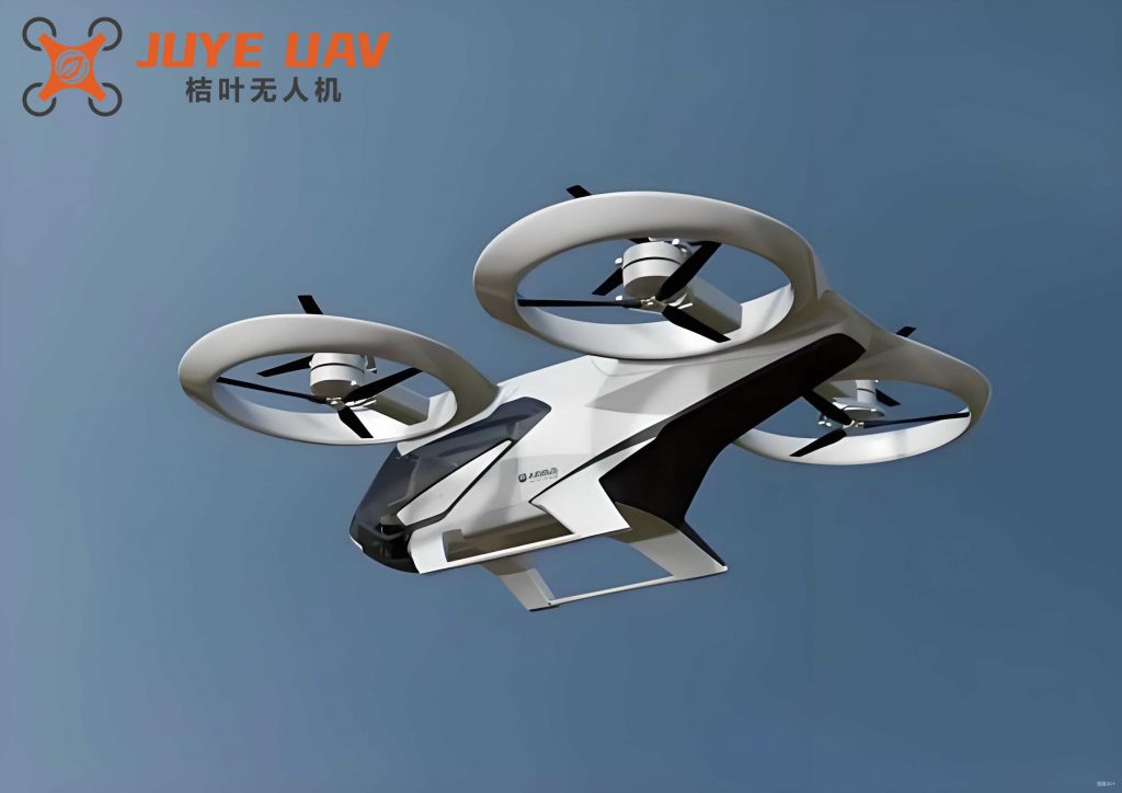
The foundation of our controller design is a potential function-based approach. For each edge in the formation graph, we define a bearing error potential energy:
$$ P_{ij}(\mathbf{r}_{ij}) = \frac{||\mathbf{g}_{ij} – \mathbf{g}_{ij}^*||^2}{||\mathbf{r}_{ij}||} $$
This function has the crucial property that it is minimized only when the bearing $\mathbf{g}_{ij}$ aligns with its desired value $\mathbf{g}_{ij}^*$. The total potential energy for drone i is the sum over its neighbors: $P_i = \sum_{j \in \mathcal{N}_i} P_{ij}$. The gradient of this potential with respect to the relative position provides a direction for corrective action:
$$ \nabla_{\mathbf{r}_{ij}} P_{ij} = \frac{\partial P_{ij}}{\partial \mathbf{r}_{ij}} = 2(\mathbf{g}_{ij} – \mathbf{g}_{ij}^*) $$
To achieve bearing-based formation stabilization while actively compensating for the unknown wind disturbances, we propose the following adaptive control and estimation laws for each quadrotor drone.
| Symbol | Description |
|---|---|
| $\mathbf{r}_i$, $\theta_i$ | Position and yaw angle of quadrotor drone i. |
| $\mathbf{v}_i$, $\omega_i$ | Nominal linear and angular velocity control inputs. |
| $\delta\mathbf{v}_i$, $\delta\omega_i$ | Unknown bounded wind disturbances. |
| $\mathbf{g}_{ij}$, $\mathbf{g}_{ij}^*$ | Actual and desired bearing vector from drone j to i. |
| $\hat{D}_{v_i}$, $\hat{D}_{\omega_i}$ | Adaptive estimates of the disturbance bounds. |
| $k_i$, $\ell_i$, $\lambda_i$, $\mu_i$ | Positive constant control and adaptation gains. |
Formation Control Law:
The control inputs for the i-th quadrotor drone are designed to descend the gradient of the potential function, with an additional robust term using the adaptive disturbance estimates.
$$ \mathbf{v}_i = -\ell_i \cdot \mathbf{R}_i^T \sum_{j \in \mathcal{N}_i} (\mathbf{g}_{ij} – \mathbf{g}_{ij}^*) – \mathbf{S}_i \hat{D}_{v_i} $$
$$ \omega_i = -k_i (\theta_i – \theta_i^*) – \hat{D}_{\omega_i} \text{sgn}(\theta_i – \theta_i^*) $$
Here, $\boldsymbol{\phi}_i = \sum_{j \in \mathcal{N}_i} (\mathbf{g}_{ij} – \mathbf{g}_{ij}^*)^T \mathbf{R}_i = [\phi_{ix}, \phi_{iy}, \phi_{iz}]$, and $\mathbf{S}_i = [\text{sgn}(\phi_{ix}), \text{sgn}(\phi_{iy}), \text{sgn}(\phi_{iz})]^T$. The sign function $\text{sgn}(\cdot)$ provides robustness against the bounded disturbance.
Adaptive Estimation Law:
To compensate for the unknown disturbance bounds $D_{v_i}$ and $D_{\omega_i}$, we employ the following update laws:
$$ \dot{\hat{D}}_{v_i} = 4\lambda_i \sum_{j \in \mathcal{N}_i} (\mathbf{g}_{ij} – \mathbf{g}_{ij}^*)^T \mathbf{R}_i \mathbf{S}_i $$
$$ \dot{\hat{D}}_{\omega_i} = \mu_i |\theta_i – \theta_i^*| $$
These estimators dynamically adjust the robust control terms based on the observed bearing and attitude errors, effectively learning the magnitude of the wind perturbations affecting each individual quadrotor drone.
| Step | Action for Quadrotor Drone i |
|---|---|
| 1. Measure | Obtain relative positions $\mathbf{r}_{ij}$ to neighbors $j \in \mathcal{N}_i$ and own yaw $\theta_i$. |
| 2. Compute | Calculate bearing vectors $\mathbf{g}_{ij}$ and errors $(\mathbf{g}_{ij} – \mathbf{g}_{ij}^*)$. Compute $\boldsymbol{\phi}_i$ and $\mathbf{S}_i$. |
| 3. Adapt | Update disturbance bound estimates $\hat{D}_{v_i}$ and $\hat{D}_{\omega_i}$ using Eq. (Adaptation Laws). |
| 4. Actuate | Apply the control inputs $\mathbf{v}_i$ and $\omega_i$ from Eq. (Control Law). |
The stability of the entire multi-quadrotor drone system under the proposed adaptive scheme is rigorously proven using Lyapunov theory and Barbalat’s lemma. We construct a composite Lyapunov function candidate:
$$ V = \sum_{i=1}^{n} P_i + \frac{1}{2}\sum_{i=1}^{n} (\theta_i – \theta_i^*)^2 + \frac{1}{2}\sum_{i=1}^{n} \left( \frac{1}{\lambda_i} \tilde{D}_{v_i}^2 + \frac{1}{\mu_i} \tilde{D}_{\omega_i}^2 \right) $$
where $\tilde{D}_{v_i} = D_{v_i} – \hat{D}_{v_i}$ and $\tilde{D}_{\omega_i} = D_{\omega_i} – \hat{D}_{\omega_i}$ are the estimation errors. Calculating the time derivative of $V$ along the trajectories of the system and substituting the control and adaptation laws yields:
$$ \dot{V} \le -4\sum_{i=1}^{n} \ell_i \left\| \sum_{j \in \mathcal{N}_i} (\mathbf{g}_{ij} – \mathbf{g}_{ij}^*) \right\|^2 – \sum_{i=1}^{n} k_i (\theta_i – \theta_i^*)^2 \le 0 $$
This demonstrates that $V$ is non-increasing and bounded below, establishing the boundedness of all signals. To prove convergence, we analyze the properties of $\dot{V}$. Since $V$ converges to a finite limit and its derivative $\dot{V}$ is uniformly continuous (as the system trajectories are bounded), Barbalat’s lemma allows us to conclude that $\dot{V} \to 0$ as $t \to \infty$. This implies:
$$ \lim_{t \to \infty} \sum_{j \in \mathcal{N}_i} (\mathbf{g}_{ij}(t) – \mathbf{g}_{ij}^*) = \mathbf{0} \quad \text{and} \quad \lim_{t \to \infty} (\theta_i(t) – \theta_i^*) = 0 $$
For a bearing rigid graph, the condition $\sum_{j \in \mathcal{N}_i} (\mathbf{g}_{ij} – \mathbf{g}_{ij}^*) = \mathbf{0}$ for all $i$ is sufficient to guarantee that $\mathbf{g}_{ij} \to \mathbf{g}_{ij}^*$ for all edges $(i,j) \in \mathcal{E}$. Therefore, the multi-quadrotor drone system globally converges to the desired bearing-rigid formation despite the persistent wind disturbances.
We validate the performance of our adaptive controller through numerical simulations involving a team of eight quadrotor drones. The communication topology is a line graph. Each drone’s dynamics include simulated wind disturbances: $\delta\mathbf{v}_i(t) = 1.2 \cdot \cos(\mathbf{v}_i)$ and $\delta\omega_i(t) = 0.1 \cdot \cos(\theta_i)$. The control and adaptation gains are set as $k_i=2$, $\ell_i=1$, $\lambda_i=0.2$, $\mu_i=0.5$, with a desired yaw $\theta_i^* = 1$ rad for all drones. The initial positions are linearly spaced.
The simulation results clearly demonstrate the effectiveness of the proposed strategy. The following table summarizes key performance metrics observed during the simulation:
| Metric | Observation | Interpretation |
|---|---|---|
| Bearing Error Convergence | $||\mathbf{g}_{ij} – \mathbf{g}_{ij}^*|| \to 0$ within ~5s. | The desired formation shape is accurately achieved. |
| Yaw Angle Convergence | $|\theta_i – \theta_i^*| \to 0$ smoothly. | All drones align to the desired orientation. |
| Disturbance Estimate | $\hat{D}_{v_i}$, $\hat{D}_{\omega_i}$ converge to steady values. | The adaptation law successfully learns and compensates for the wind bounds. |
| Trajectory Smoothness | Position and velocity profiles are continuous and oscillation-free. | The control action is robust and practical for real quadrotor drone dynamics. |
The trajectories show the drones starting from their initial collinear configuration and smoothly deploying into the final formation geometry defined solely by the bearing constraints. The linear velocities and offset angles exhibit transient activity as the formation is established, then settle to steady-state values necessary for maintaining the formation under the constant wind influence. Critically, the adaptive estimates $\hat{D}_{v_i}$ and $\hat{D}_{\omega_i}$ increase rapidly during the transient phase to counteract the disturbance, confirming that the algorithm actively compensates for the unknown wind effects. Without this adaptive component, the bearing errors would persist, preventing the accurate realization of the target formation.
In conclusion, this work presents a robust solution to the problem of bearing-based formation control for quadrotor drone swarms operating in windy conditions. By integrating a potential function derived from bearing errors with an online adaptive estimation mechanism, we have developed a distributed control law that guarantees global asymptotic stability of the desired bearing-rigid formation. The controller requires only bearing measurements (or measurements from which bearings can be computed) and does not need prior knowledge of the wind disturbance bounds. The Lyapunov-based stability proof provides strong theoretical guarantees, while simulation results confirm the practical efficacy and robustness of the approach. This adaptive framework is a significant step towards deploying reliable and resilient autonomous quadrotor drone formations in real-world environments where atmospheric disturbances are unavoidable.