
In recent years, the application of drones in entertainment and artistic displays has gained significant attention, particularly in formation drone light shows, where multiple drones coordinate to create dynamic visual patterns in the sky. The autonomous, intelligent, and clustered nature of these shows represents the future of drone technology. One of the critical challenges in formation drone light shows is the precise transformation and maintenance of formations, which can be interpreted as changes in the positions of individual drones relative to a lead drone or a virtual reference point. When a formation change is completed, each drone must achieve and maintain desired positions and velocities in the absolute coordinate system across three directions. Accurate prediction of the flight movement of the lead drone or virtual reference point is essential for ensuring smooth and responsive transitions in formation drone light shows. This article proposes a method based on a Radial Basis Function (RBF) neural network to estimate the acceleration of the lead drone or virtual reference point, enabling rapid response to maneuvering flights and minimal position and velocity deviations after formation changes. The approach incorporates an improved intelligent waterdrop algorithm to determine key parameters in the neural network, and simulations demonstrate its effectiveness in formation drone light shows under disturbances such as wind gusts and turns.
The core idea is to preemptively estimate the acceleration of the reference point, which allows the follower drones to adjust their trajectories proactively, thereby enhancing the synchronization and stability of the formation drone light show. Traditional methods often neglect the impact of acceleration changes on follower drones, focusing instead on position and velocity control. By integrating acceleration estimation into the control law, this method addresses a gap in existing research and improves the performance of formation drone light shows in dynamic environments. The RBF neural network is designed to approximate the acceleration based on position and velocity errors, while the intelligent waterdrop algorithm optimizes the network’s radial basis function centers. This combination ensures accurate estimation and robust formation keeping, even when external factors like wind disturbances are introduced during a formation drone light show.
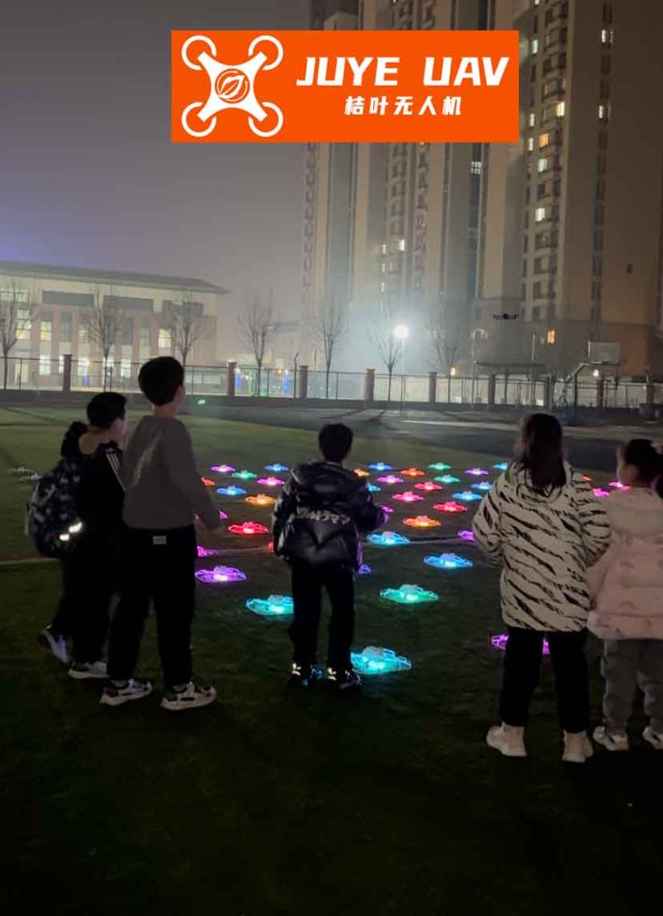
In a formation drone light show, the lead drone or virtual reference point defines the overall motion path, and follower drones must maintain specific relative positions to create visually appealing patterns. The acceleration of the reference point directly influences the followers’ dynamics, and inaccurate estimation can lead to lagging responses or formation distortions. This method leverages machine learning techniques to predict acceleration in real-time, enabling the drones to adapt quickly to changes. The RBF neural network model consists of an input layer, a hidden layer, and an output layer. The input layer receives position errors $e_i$ and velocity errors $\dot{e}_i$ for the three directions in the absolute coordinate system (i.e., $i=1,2,3$ representing x, y, and z axes). These inputs are denoted as $x_i = [e_i, \dot{e}_i]^T$. The hidden layer uses Gaussian radial basis functions to process the inputs, and the output layer produces estimated acceleration values $\hat{D}_i$ for the reference point. The neural network structure is summarized in the following table, which outlines the key components and their roles in the context of formation drone light shows.
| Component | Description | Role in Formation Drone Light Show |
|---|---|---|
| Input Layer | Receives position and velocity errors $x_i = [e_i, \dot{e}_i]^T$ | Monitors deviations of follower drones from desired patterns |
| Hidden Layer | Uses Gaussian radial basis functions $h_{ij}$ | Non-linear mapping for accurate acceleration prediction |
| Output Layer | Produces estimated acceleration $\hat{D}_i$ | Provides preemptive control input for formation maintenance |
| Radial Basis Function Centers | Determined by intelligent waterdrop algorithm | Optimizes neural network performance for dynamic shows |
The Gaussian radial basis function for the hidden layer is defined as:
$$ h_{ij} = f(x_i(k)) = \exp\left(-\frac{\sum_{k=1}^{2} \| x_i(k) – c_{\cdot j}(k) \|^2}{2\sigma_i(k)^2}\right) $$
where $i = 1,2,3$ (for three directions), $j = 1,2,\dots,7$ (for seven hidden neurons, a preset value), and $k = 1,2$ (for position and velocity errors). The vector $c_{\cdot j}$ represents the center of the radial basis function from the matrix $C$, which is a $2 \times 7$ matrix structured as:
$$ C = \begin{bmatrix} -c_{1\text{max}} & -c_{1\text{max}} \times 0.5 & -c_{1\text{max}} \times 0.2 & 0 & c_{1\text{max}} \times 0.2 & c_{1\text{max}} \times 0.5 & c_{1\text{max}} \\ -c_{2\text{max}} & -c_{2\text{max}} \times 0.5 & -c_{2\text{max}} \times 0.2 & 0 & c_{2\text{max}} \times 0.2 & c_{2\text{max}} \times 0.5 & c_{2\text{max}} \end{bmatrix} $$
Here, $c_{1\text{max}}$ and $c_{2\text{max}}$ are critical parameters obtained through the improved intelligent waterdrop algorithm, tailored for formation drone light shows. The spread constant $\sigma_i(k)$ is calculated as:
$$ \sigma_i(k) = \begin{cases} \frac{c_{1\text{max}}}{2p} & \text{for } k=1 \\ \frac{c_{2\text{max}}}{2p} & \text{for } k=2 \end{cases} $$
with $p=7$ being the number of hidden neurons. The output of the neural network, $\hat{D}_i$, is computed as:
$$ \hat{D}_i = \hat{W}_i^T H_i $$
where $\hat{W}_i$ is the actual weight vector updated iteratively, and $H_i$ is the matrix of radial basis function outputs. The weight update rule is designed to minimize errors in acceleration estimation, crucial for maintaining precise formations in drone light shows. The update is given by:
$$ \hat{W}_i = \hat{W}_i + \Delta \hat{W}_i, \quad \Delta \hat{W}_i = \alpha_i E_i^T K_i H_i $$
where $\alpha_i$ is the learning rate, $E_i = [e_i, \dot{e}_i]^T$ is the error vector, and $K_i = [k_{pi}, k_{di}]^T$ are preset proportional and derivative coefficients. This adaptive mechanism ensures that the neural network continuously improves its estimates during the formation drone light show, enhancing responsiveness to sudden movements.
To determine the optimal values of $c_{1\text{max}}$ and $c_{2\text{max}}$, an improved intelligent waterdrop algorithm is employed. In this algorithm, waterdrops simulate the drones in a formation drone light show, with their velocities and accelerations mimicking those of the drones. The algorithm iteratively explores a grid representing possible parameter values, updating soil content based on position and velocity deviations. The steps are as follows: (1) Define a training trajectory for the waterdrops and set iteration stop conditions. (2) Initialize a soil grid with boundaries based on preset maximum values for $c_{1\text{max}}$ and $c_{2\text{max}}$, assigning initial soil content to each grid cell. (3) Initialize waterdrop parameters, including number $M$, random positions on the training trajectory, and random velocities and accelerations within drone operational ranges. (4) Compute the probability $p(u,v)_k$ for a waterdrop at grid cell $u$ to move to cell $v$:
$$ p(u,v)_k = \begin{cases} \frac{\chi_s f(\text{soil}(u,v)_k)}{\sum_{\phi} f(\text{soil}(u,v)_k)} + \frac{\chi_d \left( \frac{1}{\sum_{m=1}^M \| X_{m,k}^v \|} \right)}{\sum_{\phi} \left( \frac{1}{\sum_{m=1}^M \| X_{m,k}^v \|} \right)}, & v \in \phi \\ 0, & v \notin \phi \end{cases} $$
where $\chi_s$ and $\chi_d$ are algorithm parameters with $\chi_s + \chi_d = 1$, $\phi$ is the set of feasible next grid cells, $f(\text{soil}(u,v)_k) = \frac{1}{\epsilon_s + g(\text{soil}(u,v)_k)}$ with $\epsilon_s$ a small positive constant, and $g(\cdot)$ ensures non-negative soil content. The term $\| X_{m,k}^v \|$ represents the norm of the matrix formed by position and velocity errors for the $m$-th waterdrop at cell $v$, relevant to formation drone light show performance. (5) Select the next grid cell $w$ based on these probabilities. (6) Compute the change in soil content $\delta \text{soil}(u,w)_k$:
$$ \delta \text{soil}(u,w)_k = \alpha_s \sum_{m=1}^M \| X_{m,k}^w \| $$
with $\alpha_s$ as a preset parameter. (7) Update the soil content at cell $w$:
$$ \text{soil}(u,w)_k = (1 – \rho) \text{soil}(u,w)_{k-1} – \rho \delta \text{soil}(u,w)_k $$
where $\rho = 0.01$ is a decay factor. (8) Repeat until grid boundaries are reached. (9) Check if iteration stop conditions (e.g., maximum iterations) are met; if not, restart from step 3. (10) Output the $(c_{1\text{max}}, c_{2\text{max}})$ values from the grid cell with the least soil content. For a formation drone light show, the training trajectory might be a simple path like $y = 0.5x$ with acceleration bounds of $-5 \, \text{m/s}^2$ to $5 \, \text{m/s}^2$, minimum speed $35 \, \text{m/s}$, and maximum speed $80 \, \text{m/s}$. Through this process, optimal values such as $c_{1\text{max}} = 24$ and $c_{2\text{max}} = 5$ can be obtained, which are then used in the RBF neural network for acceleration estimation in formation drone light shows.
The effectiveness of this method is demonstrated through simulation experiments in a formation drone light show scenario. Consider a show with six follower drones arranged in a hexagonal formation around a virtual reference point at the center. The neural network parameters are set as follows: learning rate $\alpha = [2, 2, 2]$, $K_i = [0.65, 0.18]^T$ for $i=1,2,3$, and with $c_{1\text{max}} = 24$ and $c_{2\text{max}} = 5$, the radial basis function center matrix and spread constants are computed as shown earlier. The initial states of the drones are provided in the table below, which highlights their starting positions, velocities, and orientations for the formation drone light show.
| Drone ID | Initial Position (m) | Velocity (m/s) | Pitch Angle (°) | Yaw Angle (°) |
|---|---|---|---|---|
| UAV1 | (93.3, 75, 50) | 50 | 0 | 0 |
| UAV2 | (50, 100, 50) | 50 | 0 | 0 |
| UAV3 | (6.7, 75, 50) | 50 | 0 | 0 |
| UAV4 | (6.7, 25, 50) | 50 | 0 | 0 |
| UAV5 | (50, 0, 50) | 50 | 0 | 0 |
| UAV6 | (93.3, 25, 50) | 50 | 0 | 0 |
The target area for the formation drone light show is a hexagonal region centered at coordinates $(-763, 850, 50)$. To simulate real-world conditions, wind disturbances and turns are introduced during the flight. The wind gust model is applied in two phases: first from approximately 5 to 10 seconds after takeoff, and second from 68 to 76 seconds. The wind direction and speed vary as shown in the simulation data, with wind density $\rho_{\text{wind}} = 1.293 \, \text{kg/m}^3$. These disturbances test the robustness of the acceleration estimation method in maintaining formation integrity during a formation drone light show.
The control law for the follower drones incorporates the estimated acceleration $\hat{D}_i$ from the neural network. It is given by:
$$ N = B^{-1} ( -K_d \dot{e} – K_p e – G – \hat{D} + a ) $$
where $N = [n_1, n_2, n_3]^T$ is the overload vector in the drone body coordinate system, $B$ is the rotation matrix from body to absolute coordinates, $K_d = \text{diag}(k_{d1}, k_{d2}, k_{d3})$ and $K_p = \text{diag}(k_{p1}, k_{p2}, k_{p3})$ are derivative and proportional coefficients, $G = [0, 0, g]^T$ with $g = 9.8 \, \text{m/s}^2$, $\hat{D} = [\hat{D}_1, \hat{D}_2, \hat{D}_3]$ is the estimated acceleration of the virtual reference point, and $a$ accounts for wind disturbance loads. This control law enables the drones to adjust their trajectories based on preemptive acceleration estimates, ensuring quick recovery from disruptions in the formation drone light show.
Simulation results show that the drones successfully navigate toward the target while maintaining the hexagonal formation. When wind gusts or turns occur, the formation temporarily distorts but quickly recovers due to the accurate acceleration estimation. The acceleration profiles of the virtual reference point and follower drones in the x and y directions are plotted, revealing that acceleration changes primarily occur during disturbances and approach zero near the target area, as expected in a well-coordinated formation drone light show. Position and velocity deviations for each drone are monitored over time. The deviations peak during wind interference and turns but diminish rapidly afterward, demonstrating the method’s effectiveness. For instance, after the third turn, within 50 seconds, the position deviations reduce to centimeter-level and velocity deviations become negligible, as summarized in the following table for the formation drone light show near the target area.
| Drone ID | x-Position Error (m) | y-Position Error (m) | x-Velocity Error (m/s) | y-Velocity Error (m/s) |
|---|---|---|---|---|
| UAV1 | -0.0366 | -0.0077 | 0.0001 | -0.0004 |
| UAV2 | -0.0205 | -0.0633 | 0.0026 | 0.0048 |
| UAV3 | -0.0354 | 0.0138 | 0.0004 | 0.0002 |
| UAV4 | -0.0363 | -0.0637 | 0.0001 | 0.0055 |
| UAV5 | -0.0354 | -0.0123 | 0.0003 | -0.0014 |
| UAV6 | -0.0356 | -0.0163 | 0.0003 | 0.0015 |
The small errors indicate that the formation drone light show can maintain precise patterns even under adverse conditions. The acceleration estimation method proves crucial for this performance, as it allows the control system to anticipate movements and compensate for delays. Moreover, the use of the intelligent waterdrop algorithm to optimize neural network parameters ensures that the estimation is tailored to the specific dynamics of formation drone light shows, avoiding the need for empirical tuning or exhaustive searches.
In conclusion, this article presents a robust method for predicting flight movement in formation drone light shows by estimating the acceleration of lead drones or virtual reference points using an RBF neural network. The improved intelligent waterdrop algorithm provides an efficient way to determine radial basis function centers, enhancing the neural network’s accuracy. Simulations under wind disturbances and turns confirm that the method enables rapid response and minimal deviations, essential for high-quality formation drone light shows. The key advantages include: (1) A systematic approach to parameter optimization that avoids guesswork, (2) Accurate acceleration estimation for preemptive control, and (3) Enhanced formation keeping with reduced errors. Future work could extend this method to larger drone swarms or more complex patterns in formation drone light shows, further pushing the boundaries of aerial entertainment technology. By integrating machine learning and optimization algorithms, this approach paves the way for more dynamic and resilient formation drone light shows, captivating audiences with seamless visual displays.
The application of such advanced techniques in formation drone light shows not only improves artistic expression but also ensures safety and reliability. As drone technology evolves, methods like this will become increasingly important for managing complex formations in real-time. The synergy between neural networks and bio-inspired algorithms offers a powerful toolkit for addressing the challenges of formation drone light shows, from acceleration prediction to disturbance rejection. Ultimately, this contributes to the broader field of autonomous systems, where precise coordination is paramount. In summary, the proposed method represents a significant step forward in the design and execution of formation drone light shows, enabling stunning performances that are both technically sophisticated and visually mesmerizing.