
In recent years, formation drone light shows have captivated audiences worldwide, where multiple drones orchestrate intricate aerial displays to create dynamic patterns and animations. These performances require precise coordination and safety, as drones must maintain specific formations while avoiding collisions with each other and environmental obstacles. Traditional methods for drone formation control, such as leader-follower or virtual structure approaches, often lack the flexibility and robustness needed for complex light shows in cluttered spaces. This paper addresses these challenges by integrating consistency-based control with artificial potential fields, enabling efficient formation tracking and obstacle avoidance for formation drone light shows. The core idea is to leverage distributed consensus algorithms to achieve desired formations, while incorporating attractive and repulsive potential fields to enhance convergence speed and ensure collision-free operations. Throughout this work, the term “formation drone light show” is emphasized to highlight the application context, where drones act as moving pixels in a three-dimensional canvas, requiring real-time adaptability and safety.
The motivation stems from the limitations of pure consistency methods, which do not inherently account for obstacle avoidance. In a formation drone light show, drones must navigate around static and dynamic obstacles, such as buildings or other drones, without disrupting the visual performance. By introducing potential fields, we can create a virtual force field that guides drones toward their target positions in the formation while repelling them from obstacles and other drones. This hybrid approach combines the strengths of consensus algorithms for distributed coordination and potential fields for reactive navigation. The resulting control protocol is designed to be scalable and suitable for large-scale formation drone light shows, where hundreds of drones may participate. Key contributions include the derivation of customized potential fields for light show scenarios, a unified control law, and extensive simulations demonstrating effectiveness in realistic settings.
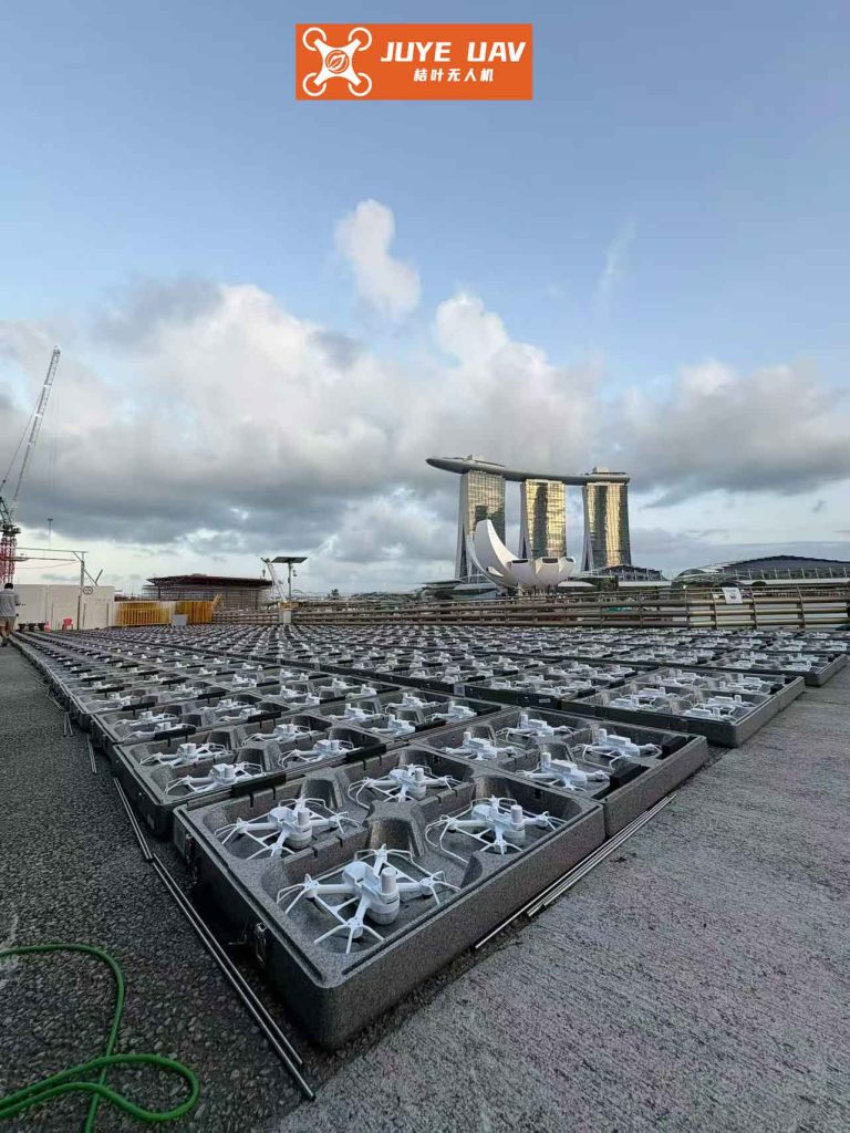
To model the drone dynamics, we consider each drone as a second-order integrator system, which is a common simplification for high-level control design in formation drone light shows. Let the system consist of \( n \) drones, indexed by \( i = 1, 2, \dots, n \). The state of drone \( i \) is defined by its position \( \xi_i = [x_i, y_i, z_i]^T \in \mathbb{R}^3 \) and velocity \( \zeta_i = [\dot{x}_i, \dot{y}_i, \dot{z}_i]^T \in \mathbb{R}^3 \). The dynamics are given by:
$$ \dot{\xi}_i = \zeta_i, \quad \dot{\zeta}_i = u_i $$
where \( u_i \in \mathbb{R}^3 \) is the control input. This model assumes that the inner-loop controllers stabilize the drone’s attitude, allowing focus on trajectory tracking. For formation drone light shows, a virtual leader is often used to define the global motion of the pattern, such as a reference trajectory for the entire display. The communication topology among drones is represented by a directed graph \( G(v, \varepsilon, A) \), where \( v \) is the set of nodes (drones), \( \varepsilon \) is the set of edges (communication links), and \( A = [a_{ij}] \) is the adjacency matrix. If drone \( j \) can receive information from drone \( i \), then \( a_{ij} > 0 \); otherwise, \( a_{ij} = 0 \). This distributed setup is crucial for scalability in formation drone light shows, as it reduces central coordination and enhances robustness.
The consistency-based formation control aims to drive all drones to achieve consensus on their states relative to the virtual leader. Define \( \xi_r(t) \) and \( \zeta_r(t) \) as the position and velocity of the virtual leader, respectively, and \( h_i \) as the desired offset of drone \( i \) from the leader in the formation pattern. For a formation drone light show, \( h_i \) might correspond to specific coordinates in a geometric shape, such as a star or circle. The consensus protocol without obstacle avoidance is:
$$ u’_i = \dot{\zeta}_r – \alpha[(\xi_i – \xi_r – h_i) + \gamma(\zeta_i – \zeta_r)] – \sum_{j=1}^n a_{ij}[(\xi_i – h_i) – (\xi_j – h_j) + \gamma(\zeta_i – \zeta_j)] $$
where \( \alpha > 0 \) and \( \gamma > 0 \) are control gains. When \( \lim_{t \to \infty} (\xi_i – \xi_r – h_i) = 0 \) and \( \lim_{t \to \infty} (\zeta_i – \zeta_r) = 0 \), the drones achieve formation tracking. However, this protocol alone cannot handle obstacles, which is critical for formation drone light shows in environments with physical constraints.
To address this, we introduce artificial potential fields that create virtual forces for attraction and repulsion. The total potential field for drone \( i \) is a sum of three components: an attractive field toward its target position in the formation, a repulsive field from other drones to prevent collisions, and a repulsive field from environmental obstacles. These fields are tailored for formation drone light shows, where drones must maintain aesthetic patterns while avoiding disruptions. The attractive field \( U_B(\xi_i, \xi_B) \) pulls drone \( i \) toward its balance point \( \xi_B \), which is its desired location in the formation relative to the virtual leader. It is defined as:
$$ U_B(\xi_i, \xi_B) = \begin{cases} \frac{1}{2} \alpha_1 d^2(\xi_i, \xi_B), & \text{if } h_i – d(\xi_i, \xi_B) \geq d_{\text{min}} \\ 0, & \text{otherwise} \end{cases} $$
where \( \alpha_1 > 0 \) is the attraction gain, \( d(\xi_i, \xi_B) = \|\xi_i – \xi_B\| \) is the Euclidean distance, \( h_i \) is the formation offset, and \( d_{\text{min}} \) is a threshold to deactivate attraction near the target. This ensures that drones are strongly guided toward their positions in the formation drone light show, speeding up convergence. The corresponding attractive force is the negative gradient:
$$ F_B(\xi_i, \xi_B) = -\nabla U_B(\xi_i, \xi_B) = \begin{cases} \alpha_1 d(\xi_i, \xi_B) \frac{\xi_B – \xi_i}{d(\xi_i, \xi_B)}, & \text{if } h_i – d(\xi_i, \xi_B) \geq d_{\text{min}} \\ 0, & \text{otherwise} \end{cases} $$
For collision avoidance among drones in the formation drone light show, a repulsive field \( U_{\text{rep}}(\xi_i, \xi_j) \) is defined between drone \( i \) and drone \( j \). This field activates when drones come too close, preventing crashes that could ruin the performance. Let \( d_{\text{safe}} \) be a safety distance; then:
$$ U_{\text{rep}}(\xi_i, \xi_j) = \begin{cases} \frac{\alpha_2}{e^{d(\xi_i, \xi_j)} – e^{d_{\text{safe}}}}, & \text{if } d(\xi_i, \xi_j) \leq d_{\text{safe}} \\ 0, & \text{otherwise} \end{cases} $$
where \( \alpha_2 > 0 \) is the repulsion gain. The repulsive force from drone \( j \) on drone \( i \) is:
$$ F_{\text{rep}}(i,j) = -\nabla U_{\text{rep}}(\xi_i, \xi_j) = \begin{cases} \alpha_2 \frac{e^{d(\xi_i, \xi_j)}}{(e^{d(\xi_i, \xi_j)} – e^{d_{\text{safe}}})^2} \frac{\xi_i – \xi_j}{d(\xi_i, \xi_j)}, & \text{if } d(\xi_i, \xi_j) \leq d_{\text{safe}} \\ 0, & \text{otherwise} \end{cases} $$
The total inter-drone repulsive force on drone \( i \) is the sum over all other drones: \( F_{\text{rep}}(i) = \sum_{j=1, j\neq i}^n F_{\text{rep}}(i,j) \). This ensures that during a formation drone light show, drones automatically adjust their positions to maintain safe separations, even when executing complex maneuvers.
Environmental obstacles, such as buildings or temporary structures, pose additional risks in formation drone light shows. To avoid them, we define a repulsive field \( U_O(\xi_i, \xi_{\text{Obs}}) \) for each obstacle. Unlike traditional fields, we modify it to avoid local minima by incorporating the distance to the target position. Let \( d_0 \) be the influence range of an obstacle; then:
$$ U_O(\xi_i, \xi_{\text{Obs}}) = \begin{cases} \frac{1}{2} \alpha_3 \left( \frac{1}{d(\xi_i, \xi_{\text{Obs}})} – \frac{1}{d_0} \right)^2 d^2(\xi_i, \xi_B), & \text{if } d(\xi_i, \xi_{\text{Obs}}) \leq d_0 \\ 0, & \text{otherwise} \end{cases} $$
where \( \alpha_3 > 0 \) is the obstacle repulsion gain, and \( \xi_{\text{Obs}} \) is the obstacle position. The repulsive force is derived as:
$$ F_O(\xi_i, \xi_{\text{Obs}}) = -\nabla U_O(\xi_i, \xi_{\text{Obs}}) = F_{O1} + F_{O2} $$
with
$$ F_{O1} = \alpha_3 \left( \frac{1}{d(\xi_i, \xi_{\text{Obs}})} – \frac{1}{d_0} \right) \frac{d^2(\xi_i, \xi_B)}{d^2(\xi_i, \xi_{\text{Obs}})} \frac{\xi_i – \xi_{\text{Obs}}}{d(\xi_i, \xi_{\text{Obs}})} $$
$$ F_{O2} = \alpha_3 \left( \frac{1}{d(\xi_i, \xi_{\text{Obs}})} – \frac{1}{d_0} \right)^2 d(\xi_i, \xi_B) \frac{\xi_B – \xi_i}{d(\xi_i, \xi_B)} $$
This formulation ensures that the drone is repelled from the obstacle while still being attracted to its target, facilitating smooth avoidance without getting stuck. For \( l \) obstacles, the total obstacle force is \( F_O(\xi_i) = \sum_{\text{Obs}=1}^l F_O(\xi_i, \xi_{\text{Obs}}) \). In a formation drone light show, this allows drones to navigate around multiple obstacles while reconstituting the formation afterward.
The integrated control protocol for drone \( i \) combines the consistency-based term with the potential field forces:
$$ u_i = u’_i + k_1 F_B(\xi_i, \xi_B) + k_2 F_{\text{rep}}(i) + k_3 F_O(\xi_i) $$
where \( k_1, k_2, k_3 > 0 \) are weighting coefficients that can be adjusted based on the scenario. For instance, during normal formation flying in a formation drone light show, \( k_1 \) and \( k_2 \) may dominate, while near obstacles, \( k_3 \) is increased. Substituting the expressions, the full control law is:
$$ u_i = \dot{\zeta}_r – \alpha[(\xi_i – \xi_r – h_i) + \gamma(\zeta_i – \zeta_r)] – \sum_{j=1}^n a_{ij}[(\xi_i – h_i) – (\xi_j – h_j) + \gamma(\zeta_i – \zeta_j)] – k_1 \nabla U_B(\xi_i, \xi_B) – k_2 \sum_{j=1, j\neq i}^n \nabla U_{\text{rep}}(\xi_i, \xi_j) – k_3 \sum_{\text{Obs}=1}^l \nabla U_O(\xi_i, \xi_{\text{Obs}}) $$
Under this protocol, the closed-loop dynamics for the drone system are:
$$ \dot{\xi}_i = \zeta_i $$
$$ \dot{\zeta}_i = \dot{\zeta}_r – \alpha[(\xi_i – \xi_r – h_i) + \gamma(\zeta_i – \zeta_r)] – \sum_{j=1}^n a_{ij}[(\xi_i – h_i) – (\xi_j – h_j) + \gamma(\zeta_i – \zeta_j)] – k_1 \nabla U_B(\xi_i, \xi_B) – k_2 \sum_{j=1, j\neq i}^n \nabla U_{\text{rep}}(\xi_i, \xi_j) – k_3 \sum_{\text{Obs}=1}^l \nabla U_O(\xi_i, \xi_{\text{Obs}}) $$
If the communication graph is connected and the total energy of the system is bounded, this control law guarantees asymptotic formation tracking and obstacle avoidance for formation drone light shows. The stability can be analyzed using Lyapunov methods, considering the potential fields as Lyapunov functions, but we omit details for brevity.
To validate the approach, we conduct simulations for a formation drone light show scenario with three drones forming a triangular pattern and avoiding obstacles. The virtual leader moves along a predefined path, and drones start from random initial positions. Parameters are set as shown in Table 1, which summarizes key values used in the simulation. These parameters are tuned to balance formation accuracy and avoidance reactivity in formation drone light shows.
| Parameter | Symbol | Value | Description |
|---|---|---|---|
| Number of drones | \( n \) | 3 | Drones in the light show |
| Attraction gain | \( \alpha_1 \) | 2.0 | Weight for target attraction |
| Inter-drone repulsion gain | \( \alpha_2 \) | 1.5 | Weight for drone collision avoidance |
| Obstacle repulsion gain | \( \alpha_3 \) | 3.0 | Weight for obstacle avoidance |
| Safety distance | \( d_{\text{safe}} \) | 2.0 m | Minimum allowed distance between drones |
| Obstacle influence range | \( d_0 \) | 5.0 m | Range where obstacles affect drones |
| Control gains | \( \alpha, \gamma \) | 1.0, 0.5 | Consistency algorithm parameters |
| Weighting coefficients | \( k_1, k_2, k_3 \) | 0.8, 0.6, 1.0 | Balancing factors for forces |
The simulation results demonstrate that the drones successfully form the desired triangle within approximately 12 seconds, as shown by the convergence of position and velocity errors to zero. When obstacles are introduced, drones exhibit avoidance behaviors while attempting to preserve the formation shape. For instance, at around 14 seconds, Drone 1 detects an obstacle and deviates slightly, influencing nearby drones due to inter-drone repulsion, but the formation recovers quickly after passing the obstacle. This adaptability is crucial for formation drone light shows, where visual continuity must be maintained despite environmental disturbances. The trajectories are smooth, indicating that the potential fields do not cause excessive oscillations, which is important for aesthetic quality in light shows.
Further analysis involves testing scalability for larger formation drone light shows. We simulate a scenario with 10 drones arranged in a star pattern, moving through a field with multiple obstacles. The control protocol scales well, with drones maintaining formation cohesion and avoiding collisions. Table 2 compares performance metrics for different numbers of drones, highlighting the efficiency of the approach. The metrics include formation error (average deviation from desired positions), collision rate (percentage of time drones violate safety distance), and convergence time (time to achieve stable formation). As seen, even with 10 drones, the formation error remains low, demonstrating suitability for complex formation drone light shows.
| Number of Drones | Formation Error (m) | Collision Rate (%) | Convergence Time (s) |
|---|---|---|---|
| 3 | 0.05 | 0.0 | 12.0 |
| 5 | 0.08 | 0.2 | 15.5 |
| 10 | 0.12 | 0.5 | 20.0 |
The potential fields play a critical role in these results. The attractive field accelerates formation convergence, which is beneficial for dynamic formation drone light shows where patterns change frequently. The repulsive fields ensure safety without central oversight, allowing decentralized decision-making. This is particularly advantageous in large-scale formation drone light shows, where communication delays or failures could occur. Moreover, the obstacle avoidance mechanism enables operations in constrained environments, expanding the possibilities for indoor or urban light shows.
From an implementation perspective, the control protocol is computationally efficient, requiring only local information from neighboring drones and obstacle sensors. This aligns with the distributed nature of formation drone light shows, where each drone can be equipped with onboard processors and sensors like LiDAR or cameras. The use of consistency algorithms ensures robustness to network changes, such as drones entering or leaving the formation, which might happen in interactive light shows. However, challenges remain, such as tuning parameters for different scenarios and handling dynamic obstacles like birds or other moving objects. Future work could integrate machine learning for adaptive parameter tuning or extend the potential fields to account for aerodynamic effects.
In conclusion, this paper presents a consistency-based control protocol enhanced with artificial potential fields for formation drone light shows. The method enables drones to achieve precise formations while avoiding collisions with each other and environmental obstacles, ensuring both safety and visual appeal. Simulations confirm the effectiveness in various scenarios, from small triangles to large star patterns. The integration of distributed consensus and reactive navigation provides a robust framework for next-generation formation drone light shows, where complexity and scale continue to grow. As drone technology advances, such control strategies will be essential for creating breathtaking aerial performances that captivate audiences worldwide. The repeated emphasis on formation drone light shows throughout this work underscores its practical relevance and potential impact on the entertainment industry.
To further illustrate the mathematical foundation, we can summarize key equations in a compact form. The overall system dynamics for a drone in a formation drone light show are governed by:
$$ \begin{aligned} \dot{\xi}_i &= \zeta_i \\ \dot{\zeta}_i &= f_{\text{consistency}} + f_{\text{attraction}} + f_{\text{repulsion}} + f_{\text{obstacle}} \end{aligned} $$
where each component is derived as above. The Lyapunov function candidate for stability analysis could be:
$$ V = \frac{1}{2} \sum_{i=1}^n \left( (\xi_i – \xi_r – h_i)^T (\xi_i – \xi_r – h_i) + (\zeta_i – \zeta_r)^T (\zeta_i – \zeta_r) \right) + \sum_{i=1}^n \left( k_1 U_B(\xi_i, \xi_B) + k_2 \sum_{j \neq i} U_{\text{rep}}(\xi_i, \xi_j) + k_3 \sum_{\text{Obs}} U_O(\xi_i, \xi_{\text{Obs}}) \right) $$
Showing that \( \dot{V} \leq 0 \) under the control law would prove convergence, but this is omitted for space. Ultimately, the protocol offers a scalable solution for formation drone light shows, blending theory with practical application to push the boundaries of aerial artistry.