
The proliferation of unmanned aerial vehicles (UAVs), particularly multi-rotor configurations, has revolutionized fields from aerial cinematography to precision agriculture and infrastructure inspection. Among these, the quadrotor drone stands out for its mechanical simplicity, agility, and hovering capability. However, a persistent and critical challenge that limits the performance, reliability, and mission scope of these aircraft is vibration. The inherent rotating components—the propellers and motors—generate periodic aerodynamic and inertial forces that propagate through the airframe. For a quadrotor drone, these vibrations are not merely a nuisance; they degrade the quality of payload data (e.g., blurry images from gimbaled cameras), accelerate fatigue in structural components, interfere with sensitive onboard electronics like inertial measurement units (IMUs) and flight controllers, and can even induce instability in flight control loops. Therefore, developing effective vibration suppression techniques is paramount for advancing quadrotor drone technology.
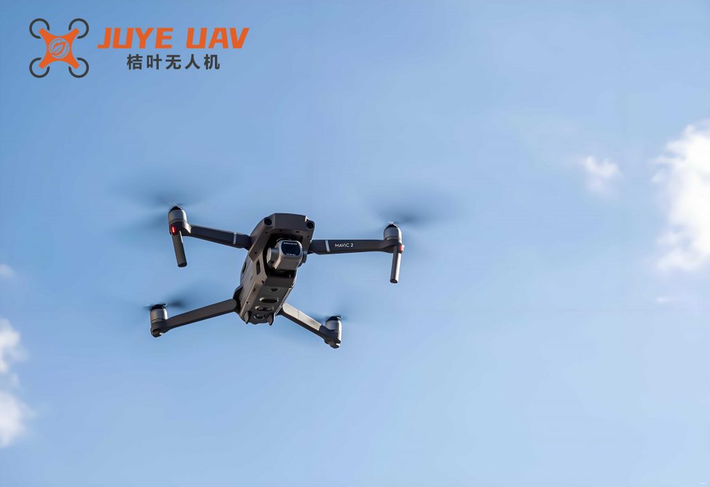
Traditional approaches to vibration control in rotary-wing aircraft often involve passive methods like vibration isolators, absorbers, or structural stiffening, and active methods such as Higher Harmonic Control (HHC) or Individual Blade Control (IBC). While effective, these methods can add significant weight, complexity, and cost, which are particularly penalizing for small to medium-sized UAVs. An alternative, inherently elegant strategy leverages the multi-source nature of the vibration itself. A quadrotor drone possesses multiple, independent vibration sources—its four rotors. By carefully controlling the relative rotational phase angles between these rotors, it is possible to exploit wave interference principles. If the vibrations transmitted from each rotor to a specific point on the fuselage can be arranged to be out of phase, destructive interference occurs, leading to a net reduction in vibration amplitude at that location. This concept of phase optimization offers a potentially massless, software-based solution for vibration suppression, requiring only precise control of motor synchronization.
This article presents a comprehensive methodology for analyzing and implementing vibration suppression in a quadrotor drone through rotor phase angle optimization. The core innovation lies in integrating a high-fidelity, coupled aeroelastic dynamics model of the full vehicle with an efficient global optimization framework based on surrogate modeling. The goal is to identify, for various steady-level flight conditions, the optimal set of phase differences between rotors that minimizes vibration at a critical payload location (e.g., a camera mount) while ensuring that vibration levels at other essential points (flight controller, arm-fuselage junctions) remain within acceptable limits. This approach moves beyond trial-and-error or simplified analytical models, providing a robust, simulation-driven design tool for vibration control in quadrotor drone systems.
1. High-Fidelity Dynamics Modeling of the Quadrotor Drone
The foundation of any reliable vibration analysis is an accurate mathematical model of the system dynamics. For a quadrotor drone, this model must capture the complex, nonlinear interactions between the four flexible rotors, their unsteady aerodynamics, and the elastic airframe. The model developed here is based on Hamilton’s principle, which provides a powerful and systematic energy-based framework for deriving equations of motion for complex dynamical systems.
The total energy functional $\Pi$ for the coupled rotor-fuselage system is considered over a time interval from $t_1$ to $t_2$. Hamilton’s principle states:
$$
\delta \Pi = \int_{t_1}^{t_2} (\delta U – \delta T – \delta W) \, dt = 0
$$
where $\delta U$ is the variation of total strain energy, $\delta T$ is the variation of total kinetic energy, and $\delta W$ is the virtual work done by external forces. For the quadrotor drone, these terms encompass contributions from all four rotors ($N_b$ blades total) and the fuselage ($F$):
$$
\delta U = \sum_{b=1}^{N_b} \delta U_b + \delta U_F, \quad \delta T = \sum_{b=1}^{N_b} \delta T_b + \delta T_F, \quad \delta W = \sum_{b=1}^{N_b} \delta W_b + \delta W_F.
$$
1.1 Rotor Blade Kinematics and Dynamics
Each rotor blade is modeled as a geometrically nonlinear, moderate-deflection beam. The position vector $\mathbf{R}_i$ of an arbitrary point on a blade of the $i$-th rotor ($i=1,2,3,4$) in the inertial frame is given by:
$$
\mathbf{R}_i = \{x_{hi}, y_{hi}, z_{hi}\}^T + \mathbf{T}_{UI}\{x+u, v, w\}^T + \mathbf{T}_{DI}\{0, \eta, \xi\}^T.
$$
Here, $\{x_{hi}, y_{hi}, z_{hi}\}$ are the coordinates of the $i$-th rotor hub. $x$ is the radial location along the undeformed blade reference line, and $u$, $v$, $w$ are the elastic deformations (axial, lag, and flap) in the blade undeformed coordinate system. $\eta$ and $\xi$ are cross-sectional coordinates. $\mathbf{T}_{UI}$ and $\mathbf{T}_{DI}$ are transformation matrices from the blade undeformed and deformed coordinate systems to the inertial frame, respectively.
Crucially, the phase angle of each rotor is incorporated into these transformations. Defining $\psi$ as the blade azimuth angle and $p_i$ as the fixed phase offset for the $i$-th rotor (with $p_1=0$ as the reference), the rotation matrix from the rotor hub to the shaft frame includes this phase:
$$
\mathbf{T}_{RH} = \begin{bmatrix}
\cos(\psi + p_i) & -\sin(\psi + p_i) & 0 \\
\sin(\psi + p_i) & \cos(\psi + p_i) & 0 \\
0 & 0 & 1
\end{bmatrix}.
$$
This ensures that the kinematic description of each rotor blade’s motion reflects its specific angular orientation relative to the others, which is fundamental to modeling their vibration superposition.
The blade kinetic energy variation $\delta T_b$ is derived from the velocity $\mathbf{V} = \dot{\mathbf{R}}_i$:
$$
\delta T_b = \int_0^R \iint_A \rho_s \mathbf{V} \cdot \delta \mathbf{V} \, d\eta \, d\zeta \, dx,
$$
where $\rho_s$ is the material density, $A$ is the cross-sectional area, and $R$ is the blade radius. The strain energy variation $\delta U_b$ is obtained from the integration of stress and strain products over the blade volume, using a constitutive relation $\{\sigma\} = [\mathbf{Q}]\{\epsilon\}$ that couples axial, torsion, and shear deformations.
1.2 Aerodynamic Modeling with Free Wake
Accurate prediction of vibratory loads requires a sophisticated aerodynamic model. A free vortex wake method is employed for each rotor. The wake is discretized into vortex filaments, and their motion is governed by:
$$
\frac{d\mathbf{r}}{dt} = \mathbf{v}(\mathbf{r}, t),
$$
where $\mathbf{r}$ is the position of a wake node and $\mathbf{v}$ is its local velocity, comprising the free-stream velocity and the induced velocities from all vortex segments in the system (including self-induction and mutual induction from other rotors). For a quadrotor drone, the mutual interference between the wakes of adjacent rotors can be significant and is fully accounted for. The induced velocity from a vortex segment is calculated using the Biot-Savart law with a viscous core model to avoid singularities:
$$
d\mathbf{v}_{ind}(\mathbf{r}) = \frac{\Gamma}{4\pi} \frac{d\mathbf{l} \times \mathbf{r}}{|\mathbf{r}|^3}.
$$
The unsteady blade airloads are then computed using a blade element approach, where the sectional velocities include components from blade motion, vehicle motion, and the inflow calculated from this detailed wake model.
1.3 Fuselage Dynamics and System Coupling
The fuselage of the quadrotor drone is treated as an elastic body. Its dynamics are represented in a modal coordinate system, derived from a finite element model:
$$
\mathbf{\overline{M}}_f \mathbf{\ddot{p}}_f + \mathbf{\overline{C}}_f \mathbf{\dot{p}}_f + \mathbf{\overline{K}}_f \mathbf{p}_f = \mathbf{\overline{F}}_f,
$$
where $\mathbf{\overline{M}}_f$, $\mathbf{\overline{C}}_f$, $\mathbf{\overline{K}}_f$ are diagonal modal mass, damping, and stiffness matrices, $\mathbf{p}_f$ is the vector of generalized coordinates (modal displacements), and $\mathbf{\overline{F}}_f$ is the vector of generalized forces from all four rotors acting at the hub connection points.
The final coupled aeroelastic equations of motion for the entire quadrotor drone system are assembled by discretizing the blade energy expressions using the finite element method and combining them with the fuselage modal equations via Hamilton’s principle. After modal reduction, the system can be expressed in a compact form:
$$
\begin{bmatrix}
\mathbf{M}_{tt} & \mathbf{M}_{tr} & \mathbf{M}_{te} \\
\mathbf{M}_{rt} & \mathbf{M}_{rr} & \mathbf{M}_{re} \\
\mathbf{M}_{et} & \mathbf{M}_{er} & \mathbf{M}_{ee}
\end{bmatrix}
\begin{Bmatrix}
\mathbf{\ddot{q}}_t \\ \mathbf{\ddot{q}}_r \\ \mathbf{\ddot{p}}_e
\end{Bmatrix} +
\begin{bmatrix}
\mathbf{C}_{tt} & \mathbf{C}_{tr} & \mathbf{C}_{te} \\
\mathbf{C}_{rt} & \mathbf{C}_{rr} & \mathbf{C}_{re} \\
\mathbf{C}_{et} & \mathbf{C}_{er} & \mathbf{C}_{ee}
\end{bmatrix}
\begin{Bmatrix}
\mathbf{\dot{q}}_t \\ \mathbf{\dot{q}}_r \\ \mathbf{\dot{p}}_e
\end{Bmatrix} +
\begin{bmatrix}
\mathbf{K}_{tt} & \mathbf{K}_{tr} & \mathbf{K}_{te} \\
\mathbf{K}_{rt} & \mathbf{K}_{rr} & \mathbf{K}_{re} \\
\mathbf{K}_{et} & \mathbf{K}_{er} & \mathbf{K}_{ee}
\end{bmatrix}
\begin{Bmatrix}
\mathbf{q}_t \\ \mathbf{q}_r \\ \mathbf{p}_e
\end{Bmatrix} =
\begin{Bmatrix}
\mathbf{F}_t \\ \mathbf{F}_r \\ \mathbf{F}_e
\end{Bmatrix}.
$$
Here, subscripts $t$, $r$, and $e$ denote rotor, fuselage rigid-body, and fuselage elastic degrees of freedom, respectively. The coupling matrices ($\mathbf{M}_{tr}$, $\mathbf{K}_{te}$, etc.) capture the dynamic interaction between these subsystems. This equation is solved using a time-domain finite element method to obtain the steady-state periodic vibration response of the quadrotor drone airframe for a given set of rotor phase angles and flight condition.
2. Surrogate-Based Optimization Framework
Directly coupling the high-fidelity dynamics solver with an optimization algorithm is computationally prohibitive, as a single vibration analysis for a quadrotor drone is resource-intensive. To enable efficient global exploration of the phase angle design space, a surrogate modeling approach is adopted. The relationship between the design variables (phase angles) and the response (vibration amplitudes at key locations) is approximated using a computationally cheap mathematical model.
2.1 Kriging Surrogate Model
The Kriging model, also known as Gaussian Process Regression, is chosen for its ability to model complex, nonlinear responses and provide an estimate of prediction uncertainty. It treats the unknown function $y(\mathbf{x})$ as a realization of a Gaussian stochastic process:
$$
y(\mathbf{x}) = \mathbf{f}^T(\mathbf{x}) \boldsymbol{\beta} + z(\mathbf{x}),
$$
where $\mathbf{f}^T(\mathbf{x})\boldsymbol{\beta}$ is a global trend function (often taken as a constant $\beta_0$), and $z(\mathbf{x})$ is a stationary Gaussian process with zero mean and covariance defined by:
$$
\text{Cov}[z(\mathbf{x}^{(i)}), z(\mathbf{x}^{(j)})] = \sigma^2 R(\boldsymbol{\theta}, \mathbf{x}^{(i)}, \mathbf{x}^{(j)}).
$$
Here, $\sigma^2$ is the process variance, and $R$ is a correlation function, typically chosen as a Gaussian exponential function of the distance between sample points $\mathbf{x}^{(i)}$ and $\mathbf{x}^{(j)}$.
Given $n$ sample points $\mathbf{S} = [\mathbf{s}_1, …, \mathbf{s}_n]^T$ with responses $\mathbf{Y} = [y_1, …, y_n]^T$, the Kriging predictor at a new point $\mathbf{x}$ is given by the Best Linear Unbiased Predictor (BLUP):
$$
\hat{y}(\mathbf{x}) = \beta_0 + \mathbf{r}^T(\mathbf{x}) \mathbf{R}_e^{-1} (\mathbf{Y} – \beta_0 \mathbf{F}),
$$
where $\mathbf{r}(\mathbf{x})$ is the vector of correlations between $\mathbf{x}$ and the sample points, $\mathbf{R}_e$ is the $n \times n$ correlation matrix between all sample points, and $\mathbf{F}$ is a vector of ones. The global mean $\beta_0$ is estimated as $\beta_0 = (\mathbf{F}^T \mathbf{R}_e^{-1} \mathbf{F})^{-1} \mathbf{F}^T \mathbf{R}_e^{-1} \mathbf{Y}$.
A key advantage of Kriging for optimizing quadrotor drone vibration is that it also provides the mean squared error (MSE) $\hat{s}^2(\mathbf{x})$ of the prediction, which quantifies uncertainty in unexplored regions of the design space.
2.2 Efficient Global Optimization with Adaptive Sampling
Initial Kriging models are built using a set of training samples generated by Latin Hypercube Sampling (LHS). To refine the model and guide the search toward the global optimum, an adaptive sampling strategy is employed. The Expected Improvement (EI) infill criterion is particularly effective. EI balances exploration (sampling where uncertainty is high) and exploitation (sampling where the predicted function value is low). For a minimization problem, the improvement at a point $\mathbf{x}$ is $I(\mathbf{x}) = \max(0, y_{min} – Y(\mathbf{x}))$, where $y_{min}$ is the current best-observed value. The expected value of this improvement, given the Kriging prediction $\hat{y}(\mathbf{x}) \sim \mathcal{N}(\hat{y}(\mathbf{x}), \hat{s}^2(\mathbf{x}))$, is:
$$
E[I(\mathbf{x})] =
\begin{cases}
(y_{min} – \hat{y}(\mathbf{x})) \Phi\left( \frac{y_{min} – \hat{y}(\mathbf{x})}{\hat{s}(\mathbf{x})} \right) + \hat{s}(\mathbf{x}) \phi\left( \frac{y_{min} – \hat{y}(\mathbf{x})}{\hat{s}(\mathbf{x})} \right), & \text{if } \hat{s}(\mathbf{x}) > 0 \\
0, & \text{if } \hat{s}(\mathbf{x}) = 0
\end{cases}
$$
where $\Phi(\cdot)$ and $\phi(\cdot)$ are the standard normal cumulative distribution and probability density functions, respectively. The point that maximizes $E[I(\mathbf{x})]$ is selected as the next infill point. Its true response is evaluated using the high-fidelity quadrotor drone dynamics model, and the Kriging model is updated. This process iterates until convergence.
3. Phase Angle Optimization Strategy for the Quadrotor Drone
The objective is to find the optimal phase offsets for rotors 2, 3, and 4 relative to rotor 1 that minimize vibration at a target location (e.g., camera mount) while constraining vibration at other critical locations. The optimization problem for a given flight speed is formally stated as:
Find:
$$
\mathbf{x} = \{ p_{2-1}, p_{3-1}, p_{4-1} \}
$$
to Minimize:
$$
\text{obj}(\mathbf{x}) = a_{cam,x}^2 + a_{cam,y}^2 + a_{cam,z}^2
$$
Subject to:
$$
\begin{aligned}
&0 \le p_{2-1} < 180^\circ \\
&0 \le p_{3-1} < 180^\circ \\
&0 \le p_{4-1} < 180^\circ \\
&a_{arm_i, xyz} \le 0.10g \quad \text{for } i=1,2,3,4 \\
&a_{fc, xyz} \le 0.05g
\end{aligned}
$$
Here, $a_{cam}$ is the vibration acceleration at the camera point, $a_{arm_i, xyz}$ is the resultant vibration at the $i$-th arm-fuselage junction, and $a_{fc, xyz}$ is the resultant vibration at the flight controller location. The constraint limits (0.10g, 0.05g) are example thresholds set to ensure structural integrity and control system functionality of the quadrotor drone. The design space is limited to $[0, 180^\circ)$ due to the inherent symmetry of the periodic vibration.
The overall workflow for the quadrotor drone vibration suppression is as follows:
- Model Validation: The coupled dynamics model is validated against experimental flight test data for a baseline phase configuration (e.g., all rotors in phase).
- Design of Experiments: An initial LHS sample set of phase angle combinations $\mathbf{x}$ is generated.
- High-Fidelity Analysis: For each sample, the full aeroelastic solver computes the vibration responses at all critical points on the quadrotor drone fuselage.
- Surrogate Model Construction: Separate Kriging models are built for the objective function $\text{obj}(\mathbf{x})$ and each constraint function.
- EGO Loop: The EI criterion is used to select new infill points. The dynamics model evaluates these points, and all Kriging models are updated. This loop continues until the change in the predicted optimum objective is negligible.
- Database Generation: The optimal phase set $\mathbf{x}^*$ is obtained for the specific flight condition. This process is repeated for a range of flight speeds (e.g., 18, 36, 54, 72 km/h) to create a look-up table or database of optimal phases.
This database can be embedded in the quadrotor drone‘s flight control system, allowing for real-time adjustment of motor synchronization based on flight speed, thereby providing adaptive vibration suppression.
4. Application and Results Analysis
The methodology is applied to a large-scale, variable-pitch quadrotor drone. The model’s predictive capability is first verified. Table 1 compares the natural frequencies of the drone’s arm structures obtained from ground vibration tests (GVT) and the finite element analysis (FEA) used to generate the fuselage modal model.
| Mode Description | Test (Hz) | Simulation (Hz) | Error (%) |
|---|---|---|---|
| 1st Flapwise Bending | 9.23 | 9.26 | 0.33 |
| 2nd Flapwise Bending | 9.89 | 10.34 | 4.55 |
| 1st Chordwise Bending | 9.95 | 9.89 | -0.60 |
| 2nd Chordwise Bending | 10.84 | 11.29 | 4.15 |
The excellent agreement (errors < 5%) validates the structural dynamics modeling of the quadrotor drone airframe. Furthermore, vibration levels at several points were compared between simulation and flight test for baseline (in-phase) conditions at 18, 36, and 54 km/h. The simulation predicted vibration trends and magnitudes with sufficient accuracy (within 20%), establishing confidence in the model for optimization studies.
Using the baseline model, the vibration environment was characterized. Figure 1 (conceptual) illustrates that vibration levels generally increase with flight speed. At higher speeds (e.g., 72 km/h), baseline vibrations at the camera and flight controller can exceed 0.25g, creating a hostile environment for payloads and electronics.
The surrogate-based optimization was then executed for four steady-level flight conditions. The optimization history for the camera vibration objective at 54 km/h is shown conceptually in Figure 2, demonstrating convergence within a limited number of high-fidelity evaluations. The final optimal phase sets identified for each speed are summarized in Table 2.
| Flight Speed (km/h) | Optimal Phase Angles [p1, p2, p3, p4] (°) | Camera Vibration Reduction Efficiency |
|---|---|---|
| 18 | [0, 31, 158, 76] | 81.1% |
| 36 | [0, 140, 60, 23] | 82.6% |
| 54 | [0, 99, 118, 134] | 83.8% |
| 72* | [0, 26, 78, 119] | 77.1% |
*For 72 km/h, constraint limits were relaxed to $a_{arm} \le 0.15g$, $a_{fc} \le 0.08g$ to find a feasible, high-efficiency solution.
The results are striking. The phase optimization strategy achieves remarkable vibration suppression at the target camera location, with efficiency exceeding 80% for low to medium speeds. Even at the high speed of 72 km/h, a 77.1% reduction is attained. The optimal phase combinations are distinct for each flight speed, underscoring that the complex aerodynamic interaction and changing load phasing on the quadrotor drone require a speed-dependent optimization. The successful identification of these sets validates the core premise: intelligent phasing of multiple rotors can drastically alter the fuselage’s vibrational state.
A detailed look at the directional vibration components reveals the effectiveness of the method. Let $a_x$, $a_y$, $a_z$ represent the vibration amplitudes along the forward, lateral, and vertical axes of the quadrotor drone, respectively. The reduction for each component at the camera point across speeds can be expressed as:
$$
\text{Reduction}_j(\%) = \left(1 – \frac{a_{j,opt}}{a_{j,baseline}}\right) \times 100, \quad \text{for } j = x, y, z.
$$
While the optimization targeted the overall resultant vibration, the solution typically provides substantial attenuation in all three axes simultaneously, often bringing each component below 0.05g. Similarly, vibration at the constrained locations (arm roots, flight controller) is successfully maintained within the prescribed limits, demonstrating that the optimization does not merely shift vibration problems to other critical parts of the quadrotor drone.
5. Discussion and Conclusion
This study has presented and demonstrated a rigorous, simulation-driven framework for suppressing vibrations in a quadrotor drone through rotor phase angle optimization. The integration of a high-fidelity, coupled aeroelastic dynamics model with an efficient Kriging-based Expected Improvement global optimization algorithm forms the core of this approach. The methodology provides several key advantages for quadrotor drone design and control:
- High Performance: It achieves dramatic vibration reduction (>80%) at targeted payload locations without adding physical mass or complex mechanisms, directly enhancing mission capability (e.g., image quality) and component longevity.
- Adaptability: By generating a database of optimal phases for different flight states, the quadrotor drone can implement adaptive, speed-dependent vibration control in real-time.
- System-Wide Consideration: The formulation includes constraints on other critical points, ensuring the solution is viable for the overall airframe integrity and control system stability of the quadrotor drone.
- Computational Efficiency: The surrogate modeling strategy makes exploring the vast design space of phase combinations feasible, transforming an intractable problem into a manageable one.
The physical principle is rooted in destructive interference. The vibrations from the four rotors propagate through different structural paths to a given point. By tuning the relative source phases ($p_i$), the arriving wavefronts can be made to cancel each other out. The optimal phases are not intuitive (e.g., simple 90° offsets) due to the asymmetry of the airflow in forward flight, the dynamic coupling between rotors through their wakes and the elastic airframe, and the differing transfer paths. This complexity necessitates the advanced numerical approach described.
It is important to note that while “zero vibration” is theoretically possible under ideal conditions, practical limitations such as slight manufacturing asymmetries, varying aerodynamic conditions, and non-identical transfer paths prevent perfect cancellation. Nevertheless, the achieved reductions are profoundly significant from an engineering standpoint.
Future work on this technology for quadrotor drone applications could focus on several areas: experimental validation of the predicted optimal phases in flight tests, extension of the optimization to include transitional maneuvers (e.g., climb, descent, turns), investigation of online adaptive algorithms that adjust phases based on real-time vibration sensor feedback, and application to more complex multi-rotor or eVTOL configurations.
In conclusion, rotor phase optimization emerges as a powerful, lightweight, and software-centric paradigm for active vibration control in quadrotor drone systems. By treating the multiple rotors not just as sources of thrust but also as actuators for vibration cancellation, this method opens a new direction for enhancing the performance and expanding the operational envelope of multi-rotor aircraft. The integrated modeling and optimization framework provides a essential tool for realizing this potential in the design and operation of advanced quadrotor drone platforms.