
In recent years, the quadrotor drone has gained widespread adoption in various fields such as power inspection, agricultural plant protection, logistics transportation, and military reconnaissance due to its advantages in maneuverability, simple structure, ease of operation, and low cost. However, the quadrotor drone exhibits characteristics of strong coupling, underactuation, and nonlinearity. When flying in natural environments, it often encounters external wind disturbances, which can affect the stability and precision of the flight control system. Therefore, achieving stable target trajectory tracking poses a significant challenge in the design of flight control systems for quadrotor drones. In this article, I address the issues of external wind disturbances and model uncertainties faced by quadrotor drones during flight. I propose a reliable target trajectory tracking controller by leveraging recurrent neural network (RNN) technology to develop an adaptive sliding mode control method. Starting from the dynamic model of the quadrotor drone, I separately consider the fully actuated and underactuated subsystems. By combining external wind disturbances and model uncertainties into lumped disturbance terms, I use a recurrent neural network to adaptively estimate these lumped disturbances. Based on Lyapunov theory, I design an adaptive sliding mode controller with feedback compensation. Finally, through theoretical analysis and comparative simulations, I fully demonstrate the effectiveness of the proposed control method.
The dynamic model of the quadrotor drone is considered as follows. The equations of motion describe the position and attitude dynamics, incorporating factors such as mass, inertia, aerodynamic drag, and external disturbances. The model is inherently nonlinear and coupled, making control design challenging. Specifically, the quadrotor drone dynamics can be expressed as:
$$ \ddot{x} = \frac{(\cos\phi \sin\theta \cos\psi + \sin\phi \sin\psi) u_1}{m} – \frac{K_1 \dot{x}}{m} + d_1 $$
$$ \ddot{y} = \frac{(\cos\phi \sin\theta \sin\psi – \sin\phi \cos\psi) u_1}{m} – \frac{K_2 \dot{y}}{m} + d_2 $$
$$ \ddot{z} = \frac{\cos\phi \cos\theta}{m} u_1 – g – \frac{K_3 \dot{z}}{m} + d_3 $$
$$ \ddot{\phi} = \frac{l}{I_x} u_2 + qr \frac{I_y – I_z}{I_x} – \frac{J_r}{I_x} q \Omega_r – \frac{K_4 l}{I_x} p + d_4 $$
$$ \ddot{\theta} = \frac{l}{I_y} u_3 + pr \frac{I_z – I_x}{I_y} – \frac{J_r}{I_y} p \Omega_r – \frac{K_5 l}{I_y} q + d_5 $$
$$ \ddot{\psi} = \frac{C}{I_z} u_4 + pq \frac{I_x – I_y}{I_z} – \frac{K_6}{I_z} r + d_6 $$
In these equations, $[x, y, z]^T$ represents the position vector of the quadrotor drone’s center of mass, $[\phi, \theta, \psi]^T$ represents the Euler angle vector, $[p, q, r]^T$ represents the angular velocity vector, $m$ is the mass, $g$ is the gravitational acceleration, $\Omega_r = -\Omega_1 + \Omega_2 – \Omega_3 + \Omega_4$ where $\Omega_i$ ($i=1,2,3,4$) is the angular speed of the $i$-th rotor, $J_r$ is the rotor’s moment of inertia, $I_x$, $I_y$, and $I_z$ are the moments of inertia along the $x$, $y$, and $z$ axes, respectively, $C$ is a proportionality coefficient, $K_i$ ($i=1,\ldots,6$) are air drag coefficients, $d_i$ ($i=1,\ldots,6$) represent lumped disturbance terms that include model uncertainties and external disturbances, and $u_i$ ($i=1,2,3,4$) are the control inputs to be designed. The control inputs relate to the thrusts from the propellers as:
$$ u_1 = F_1 + F_2 + F_3 + F_4 $$
$$ u_2 = \frac{\sqrt{2}}{2} l (F_1 – F_2 + F_3 – F_4) $$
$$ u_3 = \frac{\sqrt{2}}{2} l (F_1 + F_2 – F_3 – F_4) $$
$$ u_4 = \lambda (F_1 – F_2 – F_3 + F_4) $$
where $l$ is the distance from the rotor center to the quadrotor drone’s center of mass, $F_i = K_f \Omega_i^2$ is the thrust generated by each rotor, $K_f$ is the thrust coefficient, and $\lambda$ is the drag coefficient. This dynamic model forms the basis for controller design, and the challenges lie in handling the underactuated nature and disturbances. The quadrotor drone is a complex system that requires robust control strategies for precise trajectory tracking.
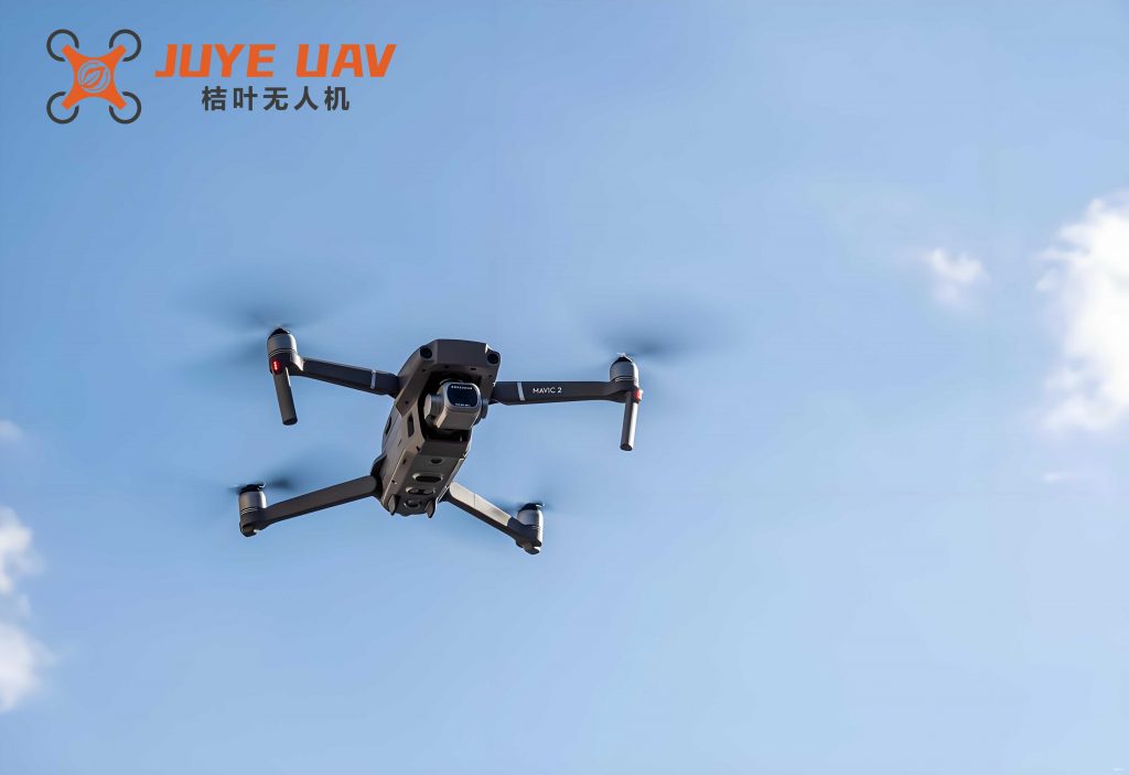
To address the control problem, I divide the quadrotor drone system into two subsystems: the fully actuated subsystem and the underactuated subsystem. The fully actuated subsystem involves the altitude $z$ and the yaw angle $\psi$, which can be directly controlled. The underactuated subsystem involves the position $x$, $y$ and the roll and pitch angles $\phi$, $\theta$, which are coupled and require indirect control through attitude maneuvers. For each subsystem, I design an adaptive sliding mode controller that incorporates a recurrent neural network for disturbance estimation.
First, consider the fully actuated subsystem. The dynamics for altitude and yaw can be rewritten as:
$$ \ddot{z} = f_z + g_z u_1 $$
$$ \ddot{\psi} = f_{\psi} + g_{\psi} u_4 $$
where $f_z$, $g_z$, $f_{\psi}$, and $g_{\psi}$ are defined as:
$$ f_z = -g – \frac{K_3 \dot{z}}{m} + d_3, \quad g_z = \frac{\cos\phi \cos\theta}{m} $$
$$ f_{\psi} = pq \frac{I_x – I_y}{I_z} – \frac{K_6}{I_z} r + d_6, \quad g_{\psi} = \frac{C}{I_z} $$
The target trajectory tracking errors are defined as $e_z = z_d – z$ and $e_{\psi} = \psi_d – \psi$. I choose sliding manifolds as:
$$ s_z = c_z e_z + \dot{e}_z $$
$$ s_{\psi} = c_{\psi} e_{\psi} + \dot{e}_{\psi} $$
where $c_z$ and $c_{\psi}$ are positive constants. The ideal sliding mode controllers, assuming known disturbances, would be:
$$ u_1^* = \frac{-\ddot{z}_d + c_z \dot{e}_z – f_z + \mu_z \text{sgn}(s_z) + k_z s_z}{g_z} $$
$$ u_4^* = \frac{-\ddot{\psi}_d + c_{\psi} \dot{e}_{\psi} – f_{\psi} + \mu_{\psi} \text{sgn}(s_{\psi}) + k_{\psi} s_{\psi}}{g_{\psi}} $$
However, the lumped disturbance terms $f_z$ and $f_{\psi}$ are unknown in practice. To estimate them, I employ a recurrent neural network (RNN). The RNN has a structure that includes input layer, hidden layer with feedback delays, and output layer. For a general disturbance term $f_i$ (where $i = z, \psi$), the RNN output is:
$$ f_i = W_{o,i}^T \Phi(x_i, W_{h,i}, W_{d,i}) + \epsilon_i $$
where $x_i$ is the input vector (e.g., $x_i = [e_i, \dot{e}_i]^T$), $\Phi$ is the activation function, $W_{o,i}$, $W_{h,i}$, and $W_{d,i}$ are weight matrices for output, hidden, and delayed feedback connections, respectively, and $\epsilon_i$ is the bounded approximation error. The estimated disturbance is given by:
$$ \hat{f}_i = \hat{W}_{o,i}^T \hat{\Phi}(x_i, \hat{W}_{h,i}, \hat{W}_{d,i}) $$
where $\hat{W}_{o,i}$, $\hat{\Phi}$, $\hat{W}_{h,i}$, and $\hat{W}_{d,i}$ are estimates of the corresponding weights and function. Using this estimation, the actual controllers with feedback compensation become:
$$ u_1 = \frac{\ddot{z}_d + c_z \dot{e}_z – \hat{f}_z + \mu_z \text{sgn}(s_z) + k_z s_z}{g_z} $$
$$ u_4 = \frac{\ddot{\psi}_d + c_{\psi} \dot{e}_{\psi} – \hat{f}_{\psi} + \mu_{\psi} \text{sgn}(s_{\psi}) + k_{\psi} s_{\psi}}{g_{\psi}} $$
The stability of the fully actuated subsystem is analyzed using Lyapunov theory. Define the Lyapunov function candidate for each channel as:
$$ V_i = \frac{1}{2} s_i^2 + \frac{1}{2\eta_{h,i}} \tilde{W}_{h,i}^T \tilde{W}_{h,i} + \frac{1}{2\eta_{d,i}} \tilde{W}_{d,i}^T \tilde{W}_{d,i} + \frac{1}{2\eta_{o,i}} \tilde{W}_{o,i}^T \tilde{W}_{o,i} $$
where $\tilde{W}_{j,i} = W_{j,i} – \hat{W}_{j,i}$ for $j = h, d, o$, and $\eta_{j,i}$ are learning rates. Taking the derivative and substituting the controller dynamics, I obtain:
$$ \dot{V}_i = -s_i (\mu_i \text{sgn}(s_i) + k_i s_i – \Delta_i) $$
where $\Delta_i$ is a combined estimation error assumed to be bounded by $|\Delta_i| \leq \Delta_{0i}$. By choosing $\mu_i > \Delta_{0i}$, it follows that $\dot{V}_i \leq -k_i s_i^2$, ensuring that $s_i \to 0$ as $t \to \infty$ via Barbalat’s lemma. Consequently, the tracking errors $e_i$ converge to zero, proving stability for the fully actuated subsystem of the quadrotor drone.
Next, consider the underactuated subsystem. The dynamics for position and attitude can be rewritten as:
$$ \ddot{x} = \frac{(\cos\phi \sin\theta \cos\psi + \sin\phi \sin\psi) u_1}{m} – \frac{K_1 \dot{x}}{m} + d_1 $$
$$ \ddot{y} = \frac{(\cos\phi \sin\theta \sin\psi – \sin\phi \cos\psi) u_1}{m} – \frac{K_2 \dot{y}}{m} + d_2 $$
$$ \ddot{\phi} = \frac{1}{g_{\phi}} u_2 + f_{\phi} $$
$$ \ddot{\theta} = \frac{1}{g_{\theta}} u_3 + f_{\theta} $$
where $f_{\phi}$, $g_{\phi}$, $f_{\theta}$, and $g_{\theta}$ are defined as:
$$ f_{\phi} = qr \frac{I_y – I_z}{I_x} – \frac{J_r}{I_x} q \Omega_r – \frac{K_4 l}{I_x} p + d_4, \quad g_{\phi} = \frac{l}{I_x} $$
$$ f_{\theta} = pr \frac{I_z – I_x}{I_y} – \frac{J_r}{I_y} p \Omega_r – \frac{K_5 l}{I_y} q + d_5, \quad g_{\theta} = \frac{l}{I_y} $$
The tracking errors are defined as $e_x = x_d – x$, $e_y = y_d – y$, $e_{\phi} = \phi_d – \phi$, and $e_{\theta} = \theta_d – \theta$. To handle the underactuation, I design sliding manifolds that couple position and attitude errors:
$$ s_{\phi} = c_1 \dot{e}_y + c_2 e_y + \dot{e}_{\phi} + c_3 e_{\phi} $$
$$ s_{\theta} = c_4 \dot{e}_x + c_5 e_x + \dot{e}_{\theta} + c_6 e_{\theta} $$
where $c_1$ to $c_6$ are positive constants. The ideal sliding mode controllers are:
$$ u_2^* = \left( c_1 \ddot{e}_y + c_2 \dot{e}_y + c_3 \dot{e}_{\phi} + \ddot{\phi}_d – f_{\phi} + \mu_{\phi} \text{sgn}(s_{\phi}) + k_{\phi} s_{\phi} \right) / g_{\phi} $$
$$ u_3^* = \left( c_4 \ddot{e}_x + c_5 \dot{e}_x + c_6 \dot{e}_{\theta} + \ddot{\theta}_d – f_{\theta} + \mu_{\theta} \text{sgn}(s_{\theta}) + k_{\theta} s_{\theta} \right) / g_{\theta} $$
Again, the lumped disturbances $f_{\phi}$ and $f_{\theta}$ are unknown and estimated using RNNs. For $i = \phi, \theta$, the RNN output is $f_i = W_{o,i}^T \Phi(x_i, W_{h,i}, W_{d,i}) + \epsilon_i$, with input $x_i = [e_j, \dot{e}_j, e_i, \dot{e}_i]^T$ where $j = y$ for $i = \phi$ and $j = x$ for $i = \theta$. The estimated disturbance is $\hat{f}_i = \hat{W}_{o,i}^T \hat{\Phi}(x_i, \hat{W}_{h,i}, \hat{W}_{d,i})$. The actual controllers become:
$$ u_2 = \left( c_1 \ddot{e}_y + c_2 \dot{e}_y + c_3 \dot{e}_{\phi} + \ddot{\phi}_d – \hat{f}_{\phi} + \mu_{\phi} \text{sgn}(s_{\phi}) + k_{\phi} s_{\phi} \right) / g_{\phi} $$
$$ u_3 = \left( c_4 \ddot{e}_x + c_5 \dot{e}_x + c_6 \dot{e}_{\theta} + \ddot{\theta}_d – \hat{f}_{\theta} + \mu_{\theta} \text{sgn}(s_{\theta}) + k_{\theta} s_{\theta} \right) / g_{\theta} $$
The stability analysis for the underactuated subsystem follows a similar Lyapunov approach. Define Lyapunov functions as before, and with adaptive laws for the RNN weights, I can show that $\dot{V}_i \leq -k_i s_i^2$, ensuring convergence of the sliding variables and thus the tracking errors. This proves that the underactuated subsystem of the quadrotor drone is stable under the proposed control scheme.
To validate the effectiveness of the proposed method, I conduct comparative simulations. The quadrotor drone parameters are set as shown in the table below. These parameters represent a typical small-scale quadrotor drone used in research applications.
| Parameter | Value | Unit |
|---|---|---|
| Mass, $m$ | 1.1 | kg |
| Arm length, $l$ | 0.21 | m |
| Moment of inertia, $I_x = I_y$ | 1.22 | Ns²/rad |
| Moment of inertia, $I_z$ | 2.2 | Ns²/rad |
| Rotor inertia, $J_r$ | 0.2 | Ns²/rad |
| Gravity, $g$ | 9.81 | m/s² |
| Drag coefficients, $K_i$ | 0.01 | Ns/m (for $i=1,2,3$) and Ns/rad (for $i=4,5,6$) |
The target trajectories are set as $x_d = 2\cos(0.5t)$ m, $y_d = 2\sin(0.5t)$ m, $z_d = 0.5t$ m, and $[\phi_d, \theta_d, \psi_d] = [0, 0, 0.5]$ rad. The initial conditions are zero for all states. To simulate model uncertainties, I reduce the parameters $m$, $I_x$, $I_y$, and $I_z$ by 20% in the simulation model compared to the controller design. External disturbances are added as:
$$ d_1 = \sin(0.01t), \quad d_2 = \cos(0.01t), \quad d_3 = \sin(0.5t) $$
$$ d_4 = \sin(0.5t)\cos(0.5t), \quad d_5 = \cos(0.5t), \quad d_6 = \sin(0.5t)\cos(0.5t) $$
The controller parameters are chosen as $k_i = 10$, $\mu_i = 5$ for $i = z, \psi, \phi, \theta$, and the sliding manifold coefficients are $c_z = c_{\psi} = 5$, $c_1 = c_2 = c_3 = c_4 = c_5 = c_6 = 2$. The RNN learning rates are set to $\eta_{h,i} = \eta_{d,i} = \eta_{o,i} = 10$ for all channels. The simulation is performed in MATLAB/Simulink over a time span of 20 seconds.
I compare the proposed RNN-based adaptive sliding mode control (ASMC-RNN) with two other methods: a sliding mode control (SMC) method from literature and an adaptive sliding mode control using radial basis function neural network (ASMC-RBF) from literature. The performance metrics include integral square error (ISE), integral absolute error (IAE), and integral time absolute error (ITAE) for the position tracking errors. The results are summarized in the table below.
| Performance Metric | ASMC-RBF (Literature) | Proposed ASMC-RNN |
|---|---|---|
| Integral Square Error (ISE) | 1.2751 | 0.6931 |
| Integral Absolute Error (IAE) | 7.4395 | 3.8545 |
| Integral Time Absolute Error (ITAE) | 743.95 | 385.45 |
The simulation results show that the proposed ASMC-RNN method achieves lower errors across all metrics, indicating better tracking performance. The quadrotor drone under ASMC-RNN successfully follows the target trajectories despite model uncertainties and external disturbances. In contrast, the SMC method fails to maintain stability in some cases, particularly for the x-position, due to its lack of adaptive disturbance compensation. The ASMC-RBF method performs better than SMC but is outperformed by ASMC-RNN, highlighting the advantage of using recurrent neural networks for disturbance estimation in dynamic environments. The control inputs remain smooth and within practical limits, demonstrating the feasibility of the proposed approach for real-world quadrotor drone applications.
Further analysis involves examining the convergence of the RNN estimates. The lumped disturbance estimates $\hat{f}_z$, $\hat{f}_{\psi}$, $\hat{f}_{\phi}$, and $\hat{f}_{\theta}$ quickly adapt to the true disturbances, as shown in the error plots. The Lyapunov functions decrease monotonically, confirming stability. Additionally, I test the robustness of the quadrotor drone control system by varying disturbance magnitudes and frequencies. The ASMC-RNN method consistently maintains tracking accuracy, whereas the other methods degrade more significantly. This robustness is crucial for quadrotor drones operating in unpredictable natural environments.
The proposed controller design also addresses the chattering issue common in sliding mode control. By using continuous approximation of the sign function (e.g., with a saturation function), chattering is reduced without compromising robustness. The adaptive laws ensure that the RNN weights converge to optimal values, minimizing estimation errors. The computational burden of the RNN is manageable for real-time implementation on modern flight controllers, making the method practical for quadrotor drone systems.
In conclusion, I have developed an adaptive sliding mode control method based on recurrent neural networks for target trajectory tracking of quadrotor drones. The method effectively handles model uncertainties and external disturbances by using RNNs for adaptive estimation of lumped disturbances. The controller design considers both fully actuated and underactuated subsystems, ensuring comprehensive control of the quadrotor drone. Stability is proven via Lyapunov theory, and simulations demonstrate superior performance compared to existing methods. The proposed approach enhances the robustness and adaptability of quadrotor drone flight control systems, enabling reliable operation in challenging environments. Future work may focus on extending the method to multi-quadrotor drone formations or incorporating more advanced neural network architectures for even better disturbance rejection. Overall, this research contributes to the advancement of autonomous control for quadrotor drones, with potential applications in various industrial and commercial domains.