
The advancement of autonomous aerial systems has propelled the quadrotor drone into a cornerstone platform for numerous applications, including surveillance, search and rescue, infrastructure inspection, and aerial cinematography. A fundamental requirement across these domains is the ability to execute precise, reliable trajectory tracking. However, the quadrotor drone presents a unique control challenge: it is an underactuated, highly coupled, and nonlinear system. Its translational motion is achieved indirectly through attitude adjustments, creating an inherent coupling between position and orientation dynamics. This complexity is significantly exacerbated by the presence of external wind disturbances. Due to their relatively low mass and flight speeds, quadrotor drones are particularly susceptible to wind gusts and turbulence, which can severely degrade tracking performance and even lead to instability. Furthermore, practical mission constraints often impose bounds on the vehicle’s attitude angles, for instance, to ensure the operational field-of-view of onboard payloads or to maintain aerodynamic efficiency. Therefore, designing a control framework that guarantees robust trajectory tracking under wind disturbances while respecting explicit attitude constraints is a critical and non-trivial problem.
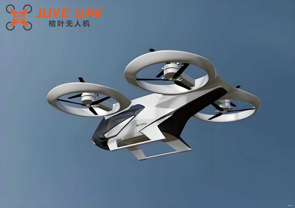
This article presents a comprehensive solution to this problem. We develop a cascaded control architecture that decouples the system into an outer-loop position subsystem and an inner-loop attitude subsystem. For the position loop, we propose a novel adaptive sliding mode controller featuring a saturated sliding surface. This design actively compensates for wind disturbances—modeled as a combination of constant and stochastic components—while ensuring that the generated attitude commands remain within predefined bounds. The adaptation mechanism estimates and pre-compensates for constant wind components, mitigating the high-frequency chattering typically associated with sliding mode control. Subsequently, an attitude extraction algorithm translates the bounded acceleration command into a feasible desired attitude, represented as a rotation matrix on the Special Orthogonal Group SO(3). For precise attitude tracking, we design a robust SO(3)-based sliding mode controller. The global stability of the entire closed-loop system is rigorously proven using Lyapunov theory. Finally, high-fidelity numerical simulations demonstrate the efficacy of the proposed controller in performing complex maneuvers, such as a spiral climb, under significant wind disturbances.
Mathematical Model of the Quadrotor Drone
We begin by establishing the dynamic model of the quadrotor drone. Let $\mathcal{I} = \{O_{\mathcal{I}}, \mathbf{e}_1, \mathbf{e}_2, \mathbf{e}_3\}$ denote an inertial, earth-fixed frame, and $\mathcal{B} = \{O_{\mathcal{B}}, \mathbf{b}_1, \mathbf{b}_2, \mathbf{b}_3\}$ denote a body-fixed frame attached to the center of mass of the drone, with $\mathbf{b}_3$ aligned with the axis of thrust. The configuration of the quadrotor drone is described by its position $\mathbf{x} \in \mathbb{R}^3$ and its attitude $\mathbf{R} \in SO(3)$, where $SO(3)$ is the Special Orthogonal Group defined as $SO(3) = \{\mathbf{R} \in \mathbb{R}^{3\times3} \, | \, \mathbf{R}^T\mathbf{R} = \mathbf{I}, \, \det(\mathbf{R}) = +1\}$. The body-fixed angular velocity is denoted by $\boldsymbol{\Omega} \in \mathbb{R}^3$.
The equations of motion for the quadrotor drone, considering wind disturbances and using the total thrust $f \in \mathbb{R}$ and the moment vector $\mathbf{M} \in \mathbb{R}^3$ as control inputs, are given by:
$$
\begin{align}
\dot{\mathbf{x}} &= \mathbf{v} \label{eq:kinematics}\\
m\dot{\mathbf{v}} &= m g \mathbf{e}_3 – f\mathbf{R}\mathbf{e}_3 + \boldsymbol{\Delta}_{\mathbf{x}} \label{eq:translation}\\
\dot{\mathbf{R}} &= \mathbf{R} \hat{\boldsymbol{\Omega}} \label{eq:att_kinematics}\\
\mathbf{J}\dot{\boldsymbol{\Omega}} &= -\boldsymbol{\Omega} \times \mathbf{J}\boldsymbol{\Omega} + \mathbf{M} \label{eq:rotation}
\end{align}
$$
Here, $m$ and $\mathbf{J} \in \mathbb{R}^{3\times3}$ are the mass and inertia matrix of the quadrotor drone, $g$ is the gravitational acceleration, and $\mathbf{v} \in \mathbb{R}^3$ is the inertial velocity. The wind disturbance force acting on the position dynamics is denoted by $\boldsymbol{\Delta}_{\mathbf{x}} \in \mathbb{R}^3$. The operator $\hat{\cdot}: \mathbb{R}^3 \to \mathfrak{so}(3)$ is the hat map, which maps a vector to a skew-symmetric matrix such that $\hat{\mathbf{a}} \mathbf{b} = \mathbf{a} \times \mathbf{b}$ for any $\mathbf{a}, \mathbf{b} \in \mathbb{R}^3$. Its inverse is the vee map $(\cdot)^\vee: \mathfrak{so}(3) \to \mathbb{R}^3$.
The wind disturbance is modeled as a superposition of a constant (or slowly varying) component and a bounded, stochastic gust component: $\boldsymbol{\Delta}_{\mathbf{x}} = \mathbf{w}_c + \mathbf{w}_d(t)$, with $\|\mathbf{w}_d(t)\| \leq \bar{w}_d$.
Control Problem Formulation
Given a sufficiently smooth desired trajectory specified by its position $\mathbf{x}_d(t)$, velocity $\mathbf{v}_d(t)$, and yaw angle $\psi_d(t)$, the control objective is to design control laws for the total thrust $f$ and moment $\mathbf{M}$ such that the quadrotor drone tracks the trajectory asymptotically, i.e., $\mathbf{x}(t) \to \mathbf{x}_d(t)$ and $\mathbf{v}(t) \to \mathbf{v}_d(t)$, despite the presence of the wind disturbance $\boldsymbol{\Delta}_{\mathbf{x}}$, and such that the generated attitude commands respect practical constraints.
We define the tracking error states for position/velocity and attitude as follows. The position and velocity errors are standard:
$$
\begin{align}
\tilde{\mathbf{x}} &= \mathbf{x} – \mathbf{x}_d \\
\tilde{\mathbf{v}} &= \mathbf{v} – \mathbf{v}_d
\end{align}
$$
For the attitude, we employ an error formulation directly on $SO(3)$. Let $\mathbf{R}_d(t) \in SO(3)$ be the desired rotation matrix (whose derivation from the position controller output will be detailed later). The attitude error function $\Psi: SO(3) \times SO(3) \to \mathbb{R}$ and the attitude error vectors $\mathbf{e}_R, \mathbf{e}_\Omega \in \mathbb{R}^3$ are defined as:
$$
\begin{align}
\Psi(\mathbf{R}, \mathbf{R}_d) &= \frac{1}{2} \text{tr}\left(\mathbf{I} – \mathbf{R}_d^T \mathbf{R}\right) \\
\mathbf{e}_R &= \frac{1}{2}\left( \mathbf{R}_d^T \mathbf{R} – \mathbf{R}^T \mathbf{R}_d \right)^\vee \\
\mathbf{e}_\Omega &= \boldsymbol{\Omega} – \mathbf{R}^T \mathbf{R}_d \boldsymbol{\Omega}_d
\end{align}
$$
where $\boldsymbol{\Omega}_d$ is the desired body angular velocity corresponding to $\mathbf{R}_d$. The time derivative of the attitude error is $\dot{\mathbf{e}}_R = \mathbf{E}(\mathbf{R}, \mathbf{R}_d) \mathbf{e}_\Omega$, where $\mathbf{E} = \frac{1}{2}\left[\text{tr}(\mathbf{R}^T\mathbf{R}_d)\mathbf{I} – \mathbf{R}^T\mathbf{R}_d\right]$ is invertible when $\Psi < 2$.
Cascaded Control Architecture
The underactuated nature of the quadrotor drone necessitates a cascaded control structure. The overall system is decomposed into two interconnected subsystems:
- Position Subsystem: Governs the translational dynamics (Eqs. \eqref{eq:kinematics}, \eqref{eq:translation}). Its output is a desired thrust vector/acceleration command.
- Attitude Subsystem: Governs the rotational dynamics (Eqs. \eqref{eq:att_kinematics}, \eqref{eq:rotation}). It must track the desired attitude generated from the position controller’s output.
The coupling between these subsystems is represented by the term $\mathbf{h} = (f/m)\mathbf{R}\mathbf{e}_3$, which is the actual thrust acceleration vector. The position controller generates a virtual control input $\mathbf{u} \in \mathbb{R}^3$, which is the desired thrust acceleration. The role of the attitude controller is then to orient the quadrotor drone such that $\mathbf{h} \to \mathbf{u}$.
| Symbol | Description | Unit |
|---|---|---|
| $\mathbf{x}, \mathbf{v}$ | Position and velocity in inertial frame | m, m/s |
| $\mathbf{R}, \boldsymbol{\Omega}$ | Attitude matrix and body angular velocity | – , rad/s |
| $m, \mathbf{J}$ | Mass and inertia matrix | kg, kg·m² |
| $f, \mathbf{M}$ | Total thrust force and control moment | N, N·m |
| $\boldsymbol{\Delta}_{\mathbf{x}}$ | Wind disturbance force | N |
| $\mathbf{u}$ | Virtual acceleration control input | m/s² |
Adaptive Sliding Mode Position Controller Design
The primary objectives of the position controller are: 1) to achieve robust tracking under wind disturbances, and 2) to ensure the generated virtual control $\mathbf{u}$ respects constraints that will later translate to bounded attitude commands.
We define a sliding surface $\mathbf{S} \in \mathbb{R}^3$ for the position subsystem:
$$
\mathbf{S} = \mathbf{P} \tilde{\mathbf{x}} + \tilde{\mathbf{v}}
$$
where $\mathbf{P} \in \mathbb{R}^{3\times3}$ is a positive definite diagonal gain matrix. To enforce output constraints, we employ a saturation function $\boldsymbol{\chi}(\mathbf{y}) = [\sigma(y_1), \sigma(y_2), \sigma(y_3)]^T$. The saturation function for the horizontal channels $(i=1,2)$ and the vertical channel $(i=3)$ are defined separately to allow for different bounds:
$$
\sigma_i(s) = \begin{cases}
s & \text{if } |s| < \delta_i, \\
\text{sgn}(s) \delta_i & \text{if } |s| \geq \delta_i,
\end{cases} \quad \text{for } i=1,2,3
$$
with $\delta_1=\delta_2$ typically. The proposed adaptive sliding mode control law for the virtual input $\mathbf{u}$ is:
$$
\begin{equation}
\mathbf{u} = g\mathbf{e}_3 – \dot{\mathbf{v}}_d + \boldsymbol{\chi}_1(\tilde{\mathbf{v}}) + \mathbf{K}_p \boldsymbol{\chi}_2(\mathbf{S}) + \boldsymbol{\chi}_3(\hat{\mathbf{w}}_c) + \mathbf{K}_s \text{sat}(\mathbf{S}/\Phi)
\end{equation}
$$
Here, $\boldsymbol{\chi}_1, \boldsymbol{\chi}_2, \boldsymbol{\chi}_3$ are saturation functions with bounds $\delta_{v}, \delta_{S}, \delta_{w}$ respectively. $\mathbf{K}_p, \mathbf{K}_s$ are positive definite diagonal gain matrices. The term $\text{sat}(\cdot)$ is a continuous saturation function used to replace the discontinuous signum function, reducing chattering, where $\Phi$ is the boundary layer thickness. The adaptive component $\hat{\mathbf{w}}_c$ is the online estimate of the constant wind disturbance $\mathbf{w}_c$, updated by the law:
$$
\dot{\hat{\mathbf{w}}}_c = \mathbf{K}_w \mathbf{S}
$$
where $\mathbf{K}_w$ is a positive definite adaptive gain matrix. Defining the estimation error as $\tilde{\mathbf{w}}_c = \hat{\mathbf{w}}_c – \mathbf{w}_c$, its dynamics become $\dot{\tilde{\mathbf{w}}}_c = \mathbf{K}_w \mathbf{S}$.
Stability Analysis (Position Loop): Consider the Lyapunov function candidate for the position subsystem:
$$
V_p = \frac{1}{2} \mathbf{S}^T \mathbf{S} + \frac{1}{2} \tilde{\mathbf{w}}_c^T \mathbf{K}_w^{-1} \tilde{\mathbf{w}}_c
$$
Its time derivative along the trajectories of the system, after substituting the control law and simplifying, can be shown to satisfy:
$$
\dot{V}_p \leq -\mathbf{S}^T \mathbf{K}_p \boldsymbol{\chi}_2(\mathbf{S}) + \mathbf{S}^T(\boldsymbol{\chi}_1(\tilde{\mathbf{v}}) – \tilde{\mathbf{v}}) + \mathbf{S}^T \mathbf{w}_d – \mathbf{S}^T \mathbf{K}_s \text{sat}(\mathbf{S}/\Phi)
$$
By assuming the stochastic disturbance is bounded, $\|\mathbf{w}_d\| \leq \bar{w}_d$, and by carefully selecting the saturation bounds $\delta_v$ and the gain $\mathbf{K}_s$ such that the minimum eigenvalue of $\mathbf{K}_s$ satisfies $\lambda_{min}(\mathbf{K}_s) > \bar{w}_d$, one can prove that $\dot{V}_p$ is negative definite outside a small neighborhood of the sliding surface $\mathbf{S} = \mathbf{0}$. According to Lyapunov theory and the properties of saturation functions, this ensures that all signals are bounded and that the tracking errors $\tilde{\mathbf{x}}$ and $\tilde{\mathbf{v}}$ converge asymptotically to zero.
| Parameter | Role |
|---|---|
| $\mathbf{P}, \mathbf{K}_p$ | Determine the dynamics of the sliding surface and error convergence. |
| $\delta_v, \delta_S, \delta_w$ | Saturation bounds for velocity error, sliding surface, and wind estimate. Constrain the virtual control $\mathbf{u}$. |
| $\mathbf{K}_s, \Phi$ | Robust gain and boundary layer for disturbance rejection and chattering reduction. |
| $\mathbf{K}_w$ | Adaptive gain for estimating constant wind component $\mathbf{w}_c$. |
Attitude Command Generation with Constraints
The virtual control $\mathbf{u}$ represents the desired inertial acceleration. The desired thrust force vector is therefore $\mathbf{F}_{des} = m\mathbf{u}$. This vector must align with the body $\mathbf{b}_3$ axis. Thus, the first step in generating the attitude command is:
$$
\mathbf{b}_{3,des} = \frac{\mathbf{F}_{des}}{\|\mathbf{F}_{des}\|}
$$
Assuming a desired yaw angle $\psi_d$ is given, we construct an intermediate vector representing the desired heading in the inertial horizontal plane: $\mathbf{b}_{yaw,des} = [\cos\psi_d, \sin\psi_d, 0]^T$. Provided $\mathbf{b}_{3,des}$ is not vertical (i.e., not parallel to $\mathbf{e}_3$), we can construct the remaining axes of the desired body frame:
$$
\begin{align}
\mathbf{b}_{2,des} &= \frac{\mathbf{b}_{3,des} \times \mathbf{b}_{yaw,des}}{\|\mathbf{b}_{3,des} \times \mathbf{b}_{yaw,des}\|} \\
\mathbf{b}_{1,des} &= \mathbf{b}_{2,des} \times \mathbf{b}_{3,des}
\end{align}
$$
The desired rotation matrix is then $\mathbf{R}_d = [\mathbf{b}_{1,des} \quad \mathbf{b}_{2,des} \quad \mathbf{b}_{3,des}] \in SO(3)$. The desired angular velocity $\boldsymbol{\Omega}_d$ and acceleration $\dot{\boldsymbol{\Omega}}_d$ can be obtained from the kinematics of $\mathbf{R}_d$.
Enforcing Attitude and Acceleration Constraints: Practical limits are often given in terms of maximum tilt (roll/pitch) angle $\theta_{max}$ and maximum vertical acceleration $a_{max}$. These constraints must be translated into bounds on the virtual control $\mathbf{u} = [u_1, u_2, u_3]^T$. The tilt angle constraint $\theta \leq \theta_{max}$ is related to the ratio of horizontal to vertical acceleration. The vertical acceleration constraint is $|u_3 – g| \leq a_{max}$. A simplified but effective set of bounds for $\mathbf{u}$ is:
$$
\begin{align}
|u_1| &\leq \frac{\sqrt{2}}{2} g \tan\theta_{max} = b_1 \\
|u_2| &\leq b_1 \\
g – a_{max} &\leq u_3 \leq g + a_{max}
\end{align}
$$
The saturation bounds $\delta_v, \delta_S, \delta_w$ and gains in the position controller (Eq. X) must be chosen conservatively to guarantee that the resulting $\mathbf{u}$ always satisfies these inequalities, ensuring the generated $\mathbf{R}_d$ is always feasible.
SO(3) Based Sliding Mode Attitude Controller
With a well-defined and bounded desired attitude $\mathbf{R}_d(t)$, the next step is to design a controller that drives $\mathbf{R}(t) \to \mathbf{R}_d(t)$ robustly. We define a sliding surface on $SO(3)$ for the attitude error dynamics:
$$
\mathbf{S}_a = \mathbf{C} \mathbf{e}_R + \mathbf{e}_\Omega
$$
where $\mathbf{C}$ is a positive definite diagonal gain matrix. The objective is to drive $\mathbf{S}_a \to \mathbf{0}$. Choosing an exponential reaching law $\dot{\mathbf{S}}_a = -\mathbf{K}_1 \mathbf{S}_a – \mathbf{K}_2 \text{sat}(\mathbf{S}_a/\Phi_a)$, and following the sliding mode control design procedure, we derive the control moment $\mathbf{M}$.
The time derivative of $\mathbf{S}_a$ is:
$$
\dot{\mathbf{S}}_a = \mathbf{C} \dot{\mathbf{e}}_R + \dot{\mathbf{e}}_\Omega = \mathbf{C}\mathbf{E}\mathbf{e}_\Omega + \mathbf{J}^{-1}(-\boldsymbol{\Omega}\times\mathbf{J}\boldsymbol{\Omega} + \mathbf{M}) – \boldsymbol{\alpha}_d
$$
where $\boldsymbol{\alpha}_d = \mathbf{R}^T\mathbf{R}_d \dot{\boldsymbol{\Omega}}_d – \widehat{\boldsymbol{\Omega}} \mathbf{R}^T\mathbf{R}_d \boldsymbol{\Omega}_d$. Setting $\dot{\mathbf{S}}_a$ equal to the desired reaching law and solving for $\mathbf{M}$ yields the SO(3) sliding mode attitude controller:
$$
\begin{equation}
\mathbf{M} = \boldsymbol{\Omega} \times \mathbf{J}\boldsymbol{\Omega} + \mathbf{J}\left[ \boldsymbol{\alpha}_d – \mathbf{E}^{-1}\left( \mathbf{C}\mathbf{E}\mathbf{e}_\Omega + \mathbf{K}_1\mathbf{S}_a + \mathbf{K}_2 \text{sat}(\mathbf{S}_a/\Phi_a) \right) \right]
\end{equation}
$$
This control law requires the inversion of $\mathbf{E}(\mathbf{R}, \mathbf{R}_d)$, which is guaranteed when the attitude error $\Psi < 2$ (i.e., before a large, $180^\circ$ error). The gains $\mathbf{K}_2$ are chosen to dominate any residual model uncertainties or disturbances in the rotational dynamics.
Stability Analysis (Attitude Loop): Consider the Lyapunov function $V_a = \frac{1}{2} \mathbf{S}_a^T \mathbf{S}_a \geq 0$. Taking its derivative and substituting the control law \eqref{eq:att_control} leads to:
$$
\dot{V}_a = \mathbf{S}_a^T \dot{\mathbf{S}}_a = -\mathbf{S}_a^T \mathbf{K}_1 \mathbf{S}_a – \mathbf{S}_a^T \mathbf{K}_2 \text{sat}(\mathbf{S}_a/\Phi_a) + \mathbf{S}_a^T \mathbf{d}
$$
where $\mathbf{d}$ represents bounded disturbances/uncertainties. By selecting $\mathbf{K}_2$ such that $\lambda_{min}(\mathbf{K}_2) > \|\mathbf{d}\|$, we ensure $\dot{V}_a < 0$ for $\mathbf{S}_a \neq \mathbf{0}$, proving the attractiveness of the sliding manifold $\mathbf{S}_a = \mathbf{0}$. On this manifold, the error dynamics become $\mathbf{C}\mathbf{e}_R + \mathbf{e}_\Omega = \mathbf{0}$, which guarantees the exponential convergence of both $\mathbf{e}_R$ and $\mathbf{e}_\Omega$ to zero. This proves almost global asymptotic stability of the desired attitude.
Numerical Simulation and Performance Evaluation
To validate the proposed control framework, we conducted high-fidelity simulations for a quadrotor drone with parameters $m = 0.455$ kg and $\mathbf{J} = \text{diag}(4.3, 4.3, 10.2) \times 10^{-3}$ kg·m². The drone was commanded to execute a demanding spiral climb trajectory defined by:
$$
\mathbf{x}_d(t) = [\sin(0.5t), \cos(0.5t), -2t]^T \, \text{m}
$$
A significant wind disturbance was introduced: $\boldsymbol{\Delta}_{\mathbf{x}} = [0.5, 0.3, 0.2]^T + \mathbf{w}_d(t)$ N, where $\mathbf{w}_d(t)$ was a vector of band-limited white noise with an RMS value of 0.25 N. Attitude constraints were set as $\theta_{max} = 30^\circ$ and $a_{max} = 0.3g$.
| Component | Parameter | Value |
|---|---|---|
| Position Controller | $\mathbf{P}$ | $\text{diag}(1.5, 1.5, 2.0)$ |
| $\mathbf{K}_p$ | $\text{diag}(2.0, 2.0, 3.0)$ | |
| $(\delta_v, \delta_S, \delta_w)$ | $(0.8, 0.5, 0.6)$ m/s, -, N | |
| $\mathbf{K}_s, \Phi$ | $\text{diag}(1.0, 1.0, 1.2)$, 0.3 | |
| Attitude Controller | $\mathbf{C}$ | $\text{diag}(3.0, 3.0, 4.0)$ |
| $\mathbf{K}_1$ | $\text{diag}(6.0, 6.0, 8.0)$ | |
| $\mathbf{K}_2, \Phi_a$ | $\text{diag}(1.5, 1.5, 2.0)$, 0.2 |
The simulation results conclusively demonstrate the effectiveness of the controller. The 3D trajectory plot shows the quadrotor drone accurately tracking the reference spiral despite the persistent wind. The initial transient deviation is quickly corrected. The position and velocity error graphs confirm asymptotic convergence, with errors settling near zero. Critically, the plots of the desired Euler angles (generated from $\mathbf{R}_d$) show that the tilt angles (roll and pitch) remain strictly within the specified $30^\circ$ limit throughout the maneuver, satisfying the operational constraint. The adaptive wind estimate $\hat{\mathbf{w}}_c$ converges rapidly to a neighborhood of the true constant wind vector $[0.5, 0.3, 0.2]^T$ N, demonstrating the efficacy of the adaptation law. The control inputs, namely the total thrust $f$ and the moments $\mathbf{M}$, remain smooth and within realistic actuation limits, with chattering effectively suppressed by the boundary layer saturation functions.
Conclusion
This article has presented a robust trajectory tracking control solution for a quadrotor drone operating in wind-disturbed environments with explicit attitude constraints. The proposed cascaded framework combines an outer-loop adaptive sliding mode position controller with an inner-loop geometric sliding mode attitude controller on $SO(3)$. The position controller innovatively integrates saturation functions within its sliding mode structure to strictly bound the virtual control command, which directly translates to bounded desired attitude angles. The adaptive component effectively estimates and compensates for constant wind biases, enhancing robustness and reducing control chattering. The $SO(3)$-based attitude controller provides almost globally stable tracking of the constrained attitude commands. Rigorous Lyapunov-based stability analysis proves the global asymptotic stability of the complete closed-loop system. Comprehensive simulation studies on a challenging spiral climb trajectory under significant stochastic and constant wind disturbances validate the theoretical results, showing precise tracking, strict constraint adherence, and smooth control signals. The proposed methodology is general and can be adapted to other underactuated aerial vehicles requiring robust, constraint-aware control in uncertain environments.