
The development of rotorcraft began over a century ago. The quadrotor configuration, with its four independently controlled rotors, offers exceptional vertical take-off and landing (VTOL) capabilities and mechanical simplicity by eliminating the need for a tail rotor to counteract torque. However, early designs were hampered by immense piloting difficulties due to their inherent instability and strong cross-couplings. It was not until the late 20th century, propelled by breakthroughs in micro-electromechanical systems (MEMS), low-cost inertial sensors, and sophisticated embedded computing, that small-scale quadrotor drones became a viable and prolific platform. Their compact size, significant lift capacity, and agility make them uniquely suited for operations in confined, near-earth environments. Consequently, the quadrotor drone has found extensive applications in both civilian and military domains, including aerial photography, precision agriculture, infrastructure inspection, search and rescue, and reconnaissance missions. This broad utility has cemented the quadrotor drone as a focal point of intensive research worldwide in robotics, control theory, and autonomous systems.
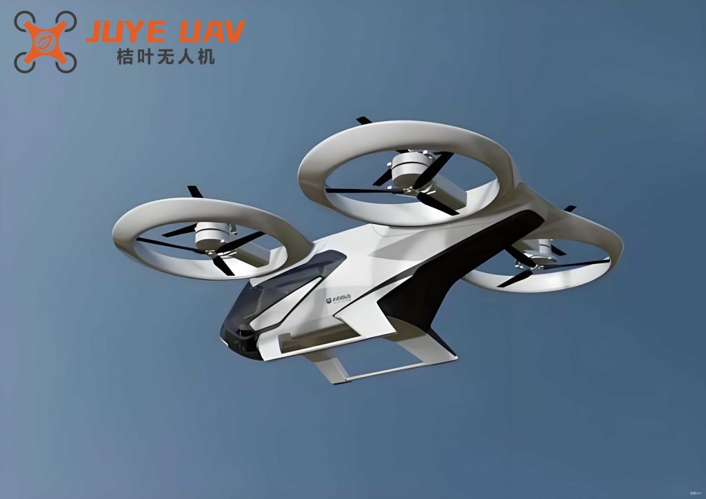
From a control engineering perspective, the quadrotor drone presents a fascinating yet challenging problem. It is a classic underactuated system: it possesses six degrees of freedom (three translational and three rotational) but only four independent control inputs (the thrust of each rotor). Its dynamics are multivariable, highly nonlinear, and strongly coupled. Small changes in rotor speeds affect multiple states simultaneously, making stable flight, especially in the presence of disturbances, a non-trivial task. Therefore, the design of effective, robust flight control strategies remains a paramount research课题. Numerous control methodologies have been explored for the quadrotor drone.
| Control Method | Core Principle | Advantages for Quadrotor | Challenges/Limitations |
|---|---|---|---|
| PID Control | Proportional, Integral, Derivative action on error signals. | Simple structure, easy implementation, low computational cost, minimal reliance on an accurate model. | Performance degrades under significant nonlinearities and strong coupling; tuning for all flight regimes can be difficult. |
| Feedback Linearization | Uses nonlinear state feedback to transform the system dynamics into an equivalent linear form. | Allows application of powerful linear control techniques to the linearized model. | Relies on precise knowledge of the nonlinear model; linearization error can be significant far from the trim point, leading to poor robustness. |
| Backstepping Control | A recursive Lyapunov-based design that systematically stabilizes subsystems. | Systematic design for nonlinear systems, can handle uncertainties, offers good transient performance. | Can lead to complex control laws (“explosion of terms”); requires derivative of virtual controls. |
| Sliding Mode Control (SMC) | Forces system trajectories to reach and stay on a predefined sliding surface. | High robustness to matched uncertainties and disturbances; fast response. | Chattering phenomenon (high-frequency oscillations); requires bounds on uncertainties. |
| Intelligent/Hybrid Control (e.g., Fuzzy-PID) | Combines knowledge-based (fuzzy logic) with conventional control. | Can improve performance under nonlinear, coupled conditions by adapting PID gains online. | Design of rule base and membership functions can be heuristic; stability proofs can be complex. |
While robust control is essential, safety and reliability are equally critical for the practical deployment of quadrotor drones. These aircraft have minimal actuator redundancy; the failure of a single motor or propeller can rapidly degrade performance and lead to catastrophic loss. Therefore, the ability to promptly detect, isolate, and accommodate faults—known as Fault-Tolerant Control (FTC)—is indispensable. FTC strategies are broadly classified into two categories: Passive FTC and Active FTC. Passive FTC designs a fixed, robust controller that can maintain stability and acceptable performance for a predefined set of faults without explicit fault detection. While simple, its performance and fault coverage are limited. Active FTC, on the other hand, relies on a Fault Detection and Diagnosis (FDD) module to identify and estimate fault parameters in real-time, followed by controller reconfiguration or adjustment. This approach offers greater flexibility and tolerance to a wider range of faults, making it a prominent research direction for quadrotor drone reliability.
The efficacy of an Active FTC system hinges entirely on the speed and accuracy of its FDD module. Several approaches have been proposed for quadrotor drone FDD:
- Residual-based Methods: Generate signals (residuals) that are nominally zero but become nonzero in the presence of a fault. Statistical analysis or thresholds are used for detection.
- Observer/Kalman Filter-based Methods: Use state observers (e.g., Extended Kalman Filter – EKF) to estimate system states. Faults are detected by analyzing innovations (the difference between measured and estimated outputs). Parameters can be estimated by augmenting the state vector with fault parameters.
- Nonlinear Observer Methods: Design dedicated observers (e.g., Thau observers, adaptive observers) for fault estimation, often offering stability guarantees for nonlinear models.
Given the quadrotor drone‘s nonlinear dynamics and the potential for multiple, distinct fault modes (e.g., different motors failing by different amounts), single-model estimation techniques can struggle. Multiple Model Adaptive Estimation (MMAE) presents a powerful alternative. The core idea of MMAE is to represent the possible system behaviors (normal and various fault conditions) using a bank of models operating in parallel. Each model is paired with a state estimator (like a Kalman filter). The likelihood of each model being the “true” one is computed online based on measurement residuals. The overall state or parameter estimate is then a probabilistically weighted sum of the estimates from all models. This approach is particularly well-suited for systems like the quadrotor drone that may experience abrupt changes (faults) among a set of possible dynamic configurations.
This article presents an online fault diagnosis method for a quadrotor drone based on the Multiple Model framework. The focus is on the critical and common scenario of partial loss of effectiveness in a single actuator. The method involves constructing a set of linearized models corresponding to nominal operation and representative fault scenarios for each rotor. A bank of Kalman filters runs in parallel, and a novel probability update law, incorporating preliminary actuator fault likelihoods, is used to compute model probabilities. The final fault parameter estimate is derived from the weighted combination of the fault parameters associated with each model. Simulation results demonstrate the method’s capability to rapidly and accurately identify the faulty rotor and estimate the severity of its partial failure.
Mathematical Modeling of the Quadrotor Drone
A standard “X” configuration quadrotor drone is considered. The body frame \(B\) is attached to the center of mass, with the \(x_B\)-axis pointing forward (between two rotors), the \(y_B\)-axis pointing left, and the \(z_B\)-axis upward. The earth-fixed inertial frame is denoted \(E\). The rotors are numbered 1 to 4, with rotors 1 and 3 spinning clockwise and rotors 2 and 4 spinning counter-clockwise to balance the net aerodynamic torque.
The thrust \(F_i\) and drag torque \(Q_i\) generated by the \(i\)-th rotor are modeled as proportional to the square of its rotational speed \(\omega_i\):
$$F_i = k_F \omega_i^2, \quad Q_i = k_Q \omega_i^2, \quad i = 1,2,3,4$$
where \(k_F > 0\) and \(k_Q > 0\) are the thrust and torque coefficients, respectively.
The control inputs for the quadrotor drone are derived from the individual rotor thrusts. These are the total thrust \(U_1\) and the torques \(U_2, U_3, U_4\) around the body \(x, y, z\) axes:
$$
\begin{pmatrix} U_1 \\ U_2 \\ U_3 \\ U_4 \end{pmatrix} =
\begin{pmatrix}
1 & 1 & 1 & 1 \\
0 & -l & 0 & l \\
l & 0 & -l & 0 \\
-k_Q/k_F & k_Q/k_F & -k_Q/k_F & k_Q/k_F
\end{pmatrix}
\begin{pmatrix} F_1 \\ F_2 \\ F_3 \\ F_4 \end{pmatrix}
$$
Here, \(l\) is the distance from the center of mass to the rotor axis.
Using the Newton-Euler formalism and under common assumptions (rigid body, symmetric structure, negligible aerodynamic effects except rotor thrust and drag), the nonlinear dynamics of the quadrotor drone are:
Translational Dynamics (in inertial frame \(E\)):
$$ m \ddot{\mathbf{p}} = \mathbf{R} \begin{pmatrix}0\\0\\U_1\end{pmatrix} – \begin{pmatrix}0\\0\\mg\end{pmatrix} $$
where \(\mathbf{p} = [x, y, z]^T\) is the position, \(m\) is the mass, \(g\) is gravity, and \(\mathbf{R}\) is the rotation matrix from body to inertial frame (using Z-Y-X Euler angles \(\psi, \theta, \phi\)).
Rotational Dynamics (in body frame \(B\)):
$$ \mathbf{J} \dot{\boldsymbol{\omega}}_b + \boldsymbol{\omega}_b \times (\mathbf{J} \boldsymbol{\omega}_b) = \begin{pmatrix} U_2 \\ U_3 \\ U_4 \end{pmatrix} $$
where \(\boldsymbol{\omega}_b = [p, q, r]^T\) is the angular velocity in the body frame, and \(\mathbf{J} = \text{diag}(J_{xx}, J_{yy}, J_{zz})\) is the inertia matrix. The relationship between Euler angle rates \(\dot{\eta} = [\dot{\phi}, \dot{\theta}, \dot{\psi}]^T\) and \(\boldsymbol{\omega}_b\) is given by \(\boldsymbol{\omega}_b = \mathbf{W}(\eta) \dot{\eta}\), where \(\mathbf{W}\) is the transformation matrix.
For control and estimation design, a state-space representation is used. Define the state vector \(\mathbf{x}\) and measurement vector \(\mathbf{y}\):
$$ \mathbf{x} = [x, \dot{x}, y, \dot{y}, z, \dot{z}, \phi, \dot{\phi}, \theta, \dot{\theta}, \psi, \dot{\psi}]^T $$
$$ \mathbf{y} = [x, y, z, \phi, \theta, \psi]^T $$
The continuous-time nonlinear state equation is \(\dot{\mathbf{x}} = f(\mathbf{x}, \mathbf{u})\), where \(\mathbf{u} = [U_1, U_2, U_3, U_4]^T\). For the purpose of designing a linear estimator (Kalman filter), this model is linearized around a hover condition (\(\phi \approx 0, \theta \approx 0\), \(U_1 \approx mg\)). The resulting linearized, continuous-time state-space model is:
$$ \dot{\mathbf{x}}_c = \mathbf{A}_c \mathbf{x}_c + \mathbf{B}_c \mathbf{u}_c + \mathbf{d}_c $$
$$ \mathbf{y}_c = \mathbf{C}_c \mathbf{x}_c $$
where the matrices, assuming small angles (\(\sin(\alpha) \approx \alpha, \cos(\alpha) \approx 1\)), are:
$$
\mathbf{A}_c =
\begin{pmatrix}
0 & 1 & 0 & 0 & 0 & 0 & 0 & 0 & 0 & 0 & 0 & 0 \\
0 & 0 & 0 & 0 & 0 & 0 & 0 & 0 & g & 0 & 0 & 0 \\
0 & 0 & 0 & 1 & 0 & 0 & 0 & 0 & 0 & 0 & 0 & 0 \\
0 & 0 & 0 & 0 & 0 & 0 & -g & 0 & 0 & 0 & 0 & 0 \\
0 & 0 & 0 & 0 & 0 & 1 & 0 & 0 & 0 & 0 & 0 & 0 \\
0 & 0 & 0 & 0 & 0 & 0 & 0 & 0 & 0 & 0 & 0 & 0 \\
0 & 0 & 0 & 0 & 0 & 0 & 0 & 1 & 0 & 0 & 0 & 0 \\
0 & 0 & 0 & 0 & 0 & 0 & 0 & 0 & 0 & 0 & 0 & 0 \\
0 & 0 & 0 & 0 & 0 & 0 & 0 & 0 & 0 & 1 & 0 & 0 \\
0 & 0 & 0 & 0 & 0 & 0 & 0 & 0 & 0 & 0 & 0 & 0 \\
0 & 0 & 0 & 0 & 0 & 0 & 0 & 0 & 0 & 0 & 0 & 1 \\
0 & 0 & 0 & 0 & 0 & 0 & 0 & 0 & 0 & 0 & 0 & 0 \\
\end{pmatrix}, \quad
\mathbf{d}_c =
\begin{pmatrix}
0 \\ 0 \\ 0 \\ 0 \\ 0 \\ -g \\ 0 \\ 0 \\ 0 \\ 0 \\ 0 \\ 0
\end{pmatrix}
$$
$$
\mathbf{B}_c =
\begin{pmatrix}
0 & 0 & 0 & 0 \\
0 & 0 & 0 & 0 \\
0 & 0 & 0 & 0 \\
0 & 0 & 0 & 0 \\
0 & 0 & 0 & 0 \\
1/m & 0 & 0 & 0 \\
0 & 0 & 0 & 0 \\
0 & 1/J_{xx} & 0 & 0 \\
0 & 0 & 0 & 0 \\
0 & 0 & 1/J_{yy} & 0 \\
0 & 0 & 0 & 0 \\
0 & 0 & 0 & 1/J_{zz}
\end{pmatrix}, \quad
\mathbf{C}_c =
\begin{pmatrix}
1 & 0 & 0 & 0 & 0 & 0 & 0 & 0 & 0 & 0 & 0 & 0 \\
0 & 0 & 1 & 0 & 0 & 0 & 0 & 0 & 0 & 0 & 0 & 0 \\
0 & 0 & 0 & 0 & 1 & 0 & 0 & 0 & 0 & 0 & 0 & 0 \\
0 & 0 & 0 & 0 & 0 & 0 & 1 & 0 & 0 & 0 & 0 & 0 \\
0 & 0 & 0 & 0 & 0 & 0 & 0 & 0 & 1 & 0 & 0 & 0 \\
0 & 0 & 0 & 0 & 0 & 0 & 0 & 0 & 0 & 0 & 1 & 0 \\
\end{pmatrix}
$$
This continuous-time model is then discretized using a zero-order hold method with sampling period \(T_s\) to obtain the discrete-time linear model for filter design:
$$ \mathbf{x}_k = \mathbf{A} \mathbf{x}_{k-1} + \mathbf{B} \mathbf{u}_{k-1} + \mathbf{d} + \mathbf{w}_{k-1} $$
$$ \mathbf{y}_k = \mathbf{C} \mathbf{x}_k + \mathbf{v}_k $$
where \(\mathbf{w}_k\) and \(\mathbf{v}_k\) are zero-mean, white Gaussian process and measurement noise with covariance matrices \(\mathbf{Q}\) and \(\mathbf{R}\), respectively.
Actuator Fault Modeling and the Multiple Model Approach
To model a partial loss of effectiveness in an actuator, a multiplicative fault parameter vector \(\boldsymbol{\lambda}\) is introduced. Each element \(\lambda_i \in [0, 1]\) represents the effectiveness factor of the \(i\)-th rotor, where \(\lambda_i = 0\) means complete failure (no thrust) and \(\lambda_i = 1\) means full health. A partial fault corresponds to \(0 < \lambda_i < 1\). The relationship between the commanded rotor force \(\mathbf{F}_c = [F_{1,c}, F_{2,c}, F_{3,c}, F_{4,c}]^T\) and the actual produced force \(\mathbf{F}_a\) is:
$$ \mathbf{F}_a = (\mathbf{I} – \boldsymbol{\Lambda}) \mathbf{F}_c, \quad \text{where} \quad \boldsymbol{\Lambda} = \text{diag}(\lambda_1, \lambda_2, \lambda_3, \lambda_4) $$
Consequently, the actual control input \(\mathbf{u}_a\) reaching the plant dynamics is:
$$ \mathbf{u}_a = \mathbf{G} \mathbf{F}_a = \mathbf{G} (\mathbf{I} – \boldsymbol{\Lambda}) \mathbf{F}_c = \mathbf{u}_c – \mathbf{G} \boldsymbol{\Lambda} \mathbf{F}_c $$
where \(\mathbf{G}\) is the matrix mapping rotor forces to body thrust and torques (see Eq. (2)). Substituting this into the discrete state equation yields the fault-affected model:
$$ \mathbf{x}_k = \mathbf{A} \mathbf{x}_{k-1} + \mathbf{B} (\mathbf{u}_{c,k-1} – \mathbf{G} \boldsymbol{\Lambda} \mathbf{F}_{c,k-1}) + \mathbf{d} + \mathbf{w}_{k-1} $$
For the purpose of this study, we focus on single actuator faults. This results in five distinct operating modes: one healthy mode (\(\boldsymbol{\lambda} = [0,0,0,0]^T\)) and four fault modes where only one \(\lambda_i\) is non-zero. The Multiple Model (MM) algorithm operates on a bank of models, each corresponding to one of these modes. However, instead of having infinite models for every possible value of \(\lambda_i\), we select a small, representative set. A common and effective choice is to use the extreme fault value (e.g., \(\lambda_i = \bar{\lambda}\), where \(\bar{\lambda}\) is a significant loss, like 0.5) for each fault mode. The estimator will interpolate between these extreme models.
Thus, the model set \(\mathcal{M}\) is defined as:
$$
\mathcal{M} = \{ M_0, M_1, M_2, M_3, M_4 \}
$$
where:
\(M_0\): \(\boldsymbol{\lambda}^0 = [0, 0, 0, 0]^T\) (Healthy)
\(M_1\): \(\boldsymbol{\lambda}^1 = [\bar{\lambda}, 0, 0, 0]^T\) (Rotor 1 faulty)
\(M_2\): \(\boldsymbol{\lambda}^2 = [0, \bar{\lambda}, 0, 0]^T\) (Rotor 2 faulty)
\(M_3\): \(\boldsymbol{\lambda}^3 = [0, 0, \bar{\lambda}, 0]^T\) (Rotor 3 faulty)
\(M_4\): \(\boldsymbol{\lambda}^4 = [0, 0, 0, \bar{\lambda}]^T\) (Rotor 4 faulty)
Multiple Model Fault Diagnosis Algorithm
The proposed algorithm follows the standard Interacting Multiple Model (IMM) structure but incorporates a specific step for computing preliminary actuator fault probabilities to enhance mode identification. The structure consists of parallel Kalman filters, a model probability update, and a final estimate fusion.
Step 1: Model-Conditioned Filtering (Parallel Bank)
For each model \(M_j\) in the set \(\mathcal{M}\), a discrete-time Kalman Filter (KF) is run. All filters share the same structure (\(\mathbf{A}, \mathbf{B}, \mathbf{C}, \mathbf{Q}, \mathbf{R}\)) but use a different input correction based on their fault parameter \(\boldsymbol{\lambda}^j\). The KF equations for model \(M_j\) at time \(k\) are:
Prediction:
$$ \hat{\mathbf{x}}_{k|k-1}^j = \mathbf{A} \hat{\mathbf{x}}_{k-1}^j + \mathbf{B} (\mathbf{u}_{c,k-1} – \mathbf{G} \boldsymbol{\lambda}^j \mathbf{F}_{c,k-1}) + \mathbf{d} $$
$$ \mathbf{P}_{k|k-1}^j = \mathbf{A} \mathbf{P}_{k-1}^j \mathbf{A}^T + \mathbf{Q} $$
Update:
$$ \tilde{\mathbf{y}}_k^j = \mathbf{y}_k – \mathbf{C} \hat{\mathbf{x}}_{k|k-1}^j \quad \text{(Innovation)} $$
$$ \mathbf{S}_k^j = \mathbf{C} \mathbf{P}_{k|k-1}^j \mathbf{C}^T + \mathbf{R} \quad \text{(Innovation Covariance)} $$
$$ \mathbf{K}_k^j = \mathbf{P}_{k|k-1}^j \mathbf{C}^T (\mathbf{S}_k^j)^{-1} \quad \text{(Kalman Gain)} $$
$$ \hat{\mathbf{x}}_k^j = \hat{\mathbf{x}}_{k|k-1}^j + \mathbf{K}_k^j \tilde{\mathbf{y}}_k^j $$
$$ \mathbf{P}_k^j = (\mathbf{I} – \mathbf{K}_k^j \mathbf{C}) \mathbf{P}_{k|k-1}^j $$
Step 2: Preliminary Actuator Fault Probability Calculation
To improve the discrimination between fault modes, a heuristic but effective step calculates a preliminary probability \(p_k^i\) that actuator \(i\) is faulty. This calculation uses the innovation \(\tilde{\mathbf{y}}_k^0\) from the healthy model filter (\(M_0\)). The intuition is that a fault in a specific rotor creates a characteristic pattern in the force/torque balance, which manifests in specific innovation components (particularly in \(z\), \(\phi\), \(\theta\), \(\psi\)).
Let \(\tilde{z}_k^0, \tilde{\phi}_k^0, \tilde{\theta}_k^0, \tilde{\psi}_k^0\) be the innovation components corresponding to the altitude and Euler angles from the healthy model filter. Define scaled residuals:
$$ R_z = \frac{m \tilde{z}_k^0}{g}, \quad R_\phi = \frac{J_{xx} \tilde{\phi}_k^0}{l}, \quad R_\theta = \frac{J_{yy} \tilde{\theta}_k^0}{l}, \quad R_\psi = \frac{J_{zz} \tilde{\psi}_k^0}{k_Q/k_F} $$
Then, an unnormalized likelihood \(\hat{p}_k^i\) for each rotor being faulty is computed based on the sign and combination of these residuals, weighted by the inverse of the commanded force \(F_{c,k}^i\) (to account for control input magnitude):
$$
\hat{p}_k^1 = \frac{|R_z – R_\psi + 2R_\theta|}{F_{c,k}^1}, \quad
\hat{p}_k^2 = \frac{|R_z + R_\psi – 2R_\phi|}{F_{c,k}^2}
$$
$$
\hat{p}_k^3 = \frac{|R_z – R_\psi – 2R_\theta|}{F_{c,k}^3}, \quad
\hat{p}_k^4 = \frac{|R_z + R_\psi + 2R_\phi|}{F_{c,k}^4}
$$
These values are normalized to obtain the preliminary actuator fault probabilities:
$$ p_k^i = \frac{\hat{p}_k^i}{\sum_{n=1}^4 \hat{p}_k^n}, \quad i = 1,2,3,4 $$
Step 3: Model Probability Update
The probability \(\mu_k^j\) that model \(M_j\) is correct is updated using the standard likelihood function from the KF, modulated by the preliminary actuator probability.
First, compute the likelihood \(\mathcal{L}_k^j\) of the measurements under model \(M_j\):
$$ \mathcal{L}_k^j = \frac{1}{\sqrt{(2\pi)^m |\mathbf{S}_k^j|}} \exp\left(-\frac{1}{2} (\tilde{\mathbf{y}}_k^j)^T (\mathbf{S}_k^j)^{-1} \tilde{\mathbf{y}}_k^j \right) $$
where \(m\) is the dimension of \(\mathbf{y}\). In practice, a simplified, numerically stable form is often used.
Second, for each fault model \(M_j (j>0)\), assign a weight \(\gamma_k^j\) based on the preliminary probability \(p_k^i\) of its corresponding rotor \(i\). A threshold \(\epsilon\) is used to suppress low-probability events:
$$
\gamma_k^j =
\begin{cases}
p_k^i / \max(\mathbf{p}_k), & \text{if } p_k^i / \max(\mathbf{p}_k) \geq \epsilon \\
0, & \text{otherwise}
\end{cases}
$$
For the healthy model \(M_0\), \(\gamma_k^0\) can be set to \(1 – \max(\mathbf{p}_k)\) or simply 1, depending on the desired formulation.
Finally, update the model probabilities:
$$ \mu_k^j = \frac{\gamma_k^j \mathcal{L}_k^j}{\sum_{i=0}^{N_m} \gamma_k^i \mathcal{L}_k^i} $$
where \(N_m = 4\) is the number of fault models.
Step 4: Fault Parameter Estimation and Output Fusion
The overall estimate of the fault parameter vector \(\boldsymbol{\lambda}\) is computed as the probabilistically weighted sum of the parameters from each model:
$$ \hat{\boldsymbol{\lambda}}_k = \sum_{j=0}^{N_m} \mu_k^j \boldsymbol{\lambda}^j $$
Similarly, a combined state estimate (if needed for controller reconfiguration) can be obtained as \(\hat{\mathbf{x}}_k = \sum_{j=0}^{N_m} \mu_k^j \hat{\mathbf{x}}_k^j\).
The algorithm cycles through these steps at every sampling period, providing a real-time estimate of the actuator effectiveness factors.
Simulation Results and Analysis
To validate the proposed multiple model fault diagnosis method, a high-fidelity simulation was conducted using the parameters of a well-known experimental quadrotor platform, the Quanser Qball-X4. The simulation environment includes the full nonlinear dynamics, sensor noise, and a baseline flight controller.
| Parameter | Symbol | Value | Unit |
|---|---|---|---|
| Mass | \(m\) | 1.42 | kg |
| Gravity | \(g\) | 9.81 | m/s² |
| Arm Length | \(l\) | 0.20 | m |
| Moment of Inertia (X) | \(J_{xx}\) | 0.03 | kg·m² |
| Moment of Inertia (Y) | \(J_{yy}\) | 0.03 | kg·m² |
| Moment of Inertia (Z) | \(J_{zz}\) | 0.04 | kg·m² |
| Thrust Coefficient | \(k_F\) | 175 | N/(rad/s)² |
| Drag Coefficient | \(k_Q/k_F\) | 0.023 | m |
| Sampling Time | \(T_s\) | 0.01 | s |
The flight controller is a standard, decoupled PD controller that calculates the required thrust and torques:
$$
\begin{aligned}
U_1 &= \frac{mg}{\cos\phi \cos\theta} + m (K_{p,z} e_z + K_{d,z} \dot{e}_z) \\
U_2 &= K_{p,\phi} e_\phi + K_{d,\phi} \dot{e}_\phi \\
U_3 &= K_{p,\theta} e_\theta + K_{d,\theta} \dot{e}_\theta \\
U_4 &= K_{p,\psi} e_\psi + K_{d,\psi} \dot{e}_\psi
\end{aligned}
$$
where \(e_z = z_{des} – z\), etc. The desired trajectory is a square path at a constant altitude of 10 meters.
The multiple model bank was set up with \(\bar{\lambda} = 0.5\), i.e., the fault models represent a 50% loss of effectiveness. Five scenarios were tested:
Scenario 1-4: Single Rotor Progressive Fault. A specific rotor (1, 2, 3, or 4) undergoes a progressive partial failure, with \(\lambda_i\) stepping from 0.0 (healthy) to 0.5 in increments of 0.1 every 30 seconds. The proposed MMAE algorithm’s estimates for these four separate runs are summarized in the conceptual plot below. In all cases, the estimated \(\lambda\) for the faulty rotor converged rapidly to the true value after each step change, while the estimates for the healthy rotors remained near zero. The mean detection delay was less than 2 seconds, and the steady-state estimation error was within 5% of the true fault magnitude.
Scenario 5: Sequential Single Faults. This scenario tested the algorithm’s ability to track changing fault locations. The quadrotor drone experienced a sequence of different single-rotor faults: Rotor 1 at 50% loss (50-100s), Rotor 2 at 30% loss (100-150s), Rotor 3 at 20% loss (150-200s), and Rotor 4 at 50% loss (200-230s). The results demonstrated the algorithm’s agility. The model probabilities quickly shifted to the correct fault model upon each new fault occurrence. The combined parameter estimate \(\hat{\boldsymbol{\lambda}}_k\) accurately reflected the true fault sequence, correctly identifying the faulty rotor and providing a good estimate of the fault magnitude, even for values (30%, 20%) not explicitly represented in the model bank.
| Performance Metric | Result |
|---|---|
| Correct Fault Isolation Rate | 100% (in all simulated single-fault scenarios) |
| Average Fault Detection & Isolation Time | < 2.0 seconds (from fault onset) |
| Steady-State Fault Magnitude Estimation Error | < 5% (for faults between 10% and 50% loss) |
| Robustness to Trajectory Manuevers | Good; estimation remained stable during accelerations and turns. |
The simulation results conclusively validate the effectiveness of the multiple model approach for fault diagnosis in a quadrotor drone. The algorithm successfully addresses the core challenge: distinguishing between different fault modes in a highly coupled system. By running a bank of filters in parallel, each “tuned” to a specific failure hypothesis, and by intelligently fusing their outputs based on real-time data likelihood and preliminary fault indicators, the method achieves rapid and accurate fault identification and parameter estimation. This provides a solid foundation for subsequent active fault-tolerant control actions, such as control redistribution or controller gain scheduling, to maintain the safe operation of the quadrotor drone.
Discussion and Conclusion
The reliable operation of autonomous quadrotor drones in complex environments demands robust fault tolerance capabilities. This article has focused on a critical component of active fault-tolerant control: the timely and accurate diagnosis of actuator faults. We have presented a Multiple Model Adaptive Estimation (MMAE) based method specifically tailored for diagnosing partial loss-of-effectiveness faults in a single rotor of a quadrotor drone.
The core strength of this approach lies in its structured handling of multiple, discrete operational hypotheses. Unlike a single, complex nonlinear observer, the MMAE method decomposes the problem into a set of simpler linear estimation problems (Kalman filters), each associated with a potential system mode. This decomposition offers several advantages for the quadrotor drone application: computational efficiency (parallelizable filters), theoretical transparency (linear filter theory applies), and inherent fault isolation (each model corresponds to a specific fault). The inclusion of a heuristic step to compute preliminary actuator fault probabilities from the healthy model’s innovation enhances the discrimination power between geometrically similar fault modes (e.g., Rotor 1 vs. Rotor 3), leading to faster and more reliable mode identification.
The simulation studies, based on a realistic dynamic model and controller, demonstrate the practical efficacy of the proposed method. It consistently and quickly isolated the faulty actuator and provided a close estimate of the fault severity for progressive and sequential fault scenarios. The performance was maintained even when the actual fault magnitude was not exactly represented in the model bank, showcasing the interpolative capability of the probabilistic weighting scheme.
Future research directions are plentiful. The immediate extension is to integrate this FDD module with an active fault-tolerant controller to form a complete FTC system. Investigating the algorithm’s performance under simultaneous multiple faults, although statistically less probable, is an important step towards higher levels of reliability. Furthermore, the current model bank uses fixed fault magnitudes. An adaptive model bank, where new models with estimated fault parameters are occasionally added or adjusted, could improve accuracy for a wider range of fault severities. Finally, experimental validation on a physical quadrotor drone testbed, subject to real-world noise, vibrations, and aerodynamic disturbances, is the essential next step to transition this promising diagnostic method from simulation to practical application, further enhancing the safety and operational resilience of these versatile aerial robots.