
The stable and precise control of a quadrotor drone is fundamental to its ability to perform a wide array of complex tasks, from aerial cinematography and precision agriculture to search and rescue operations. The core of this capability lies in its flight control system, with the low-level attitude controller being the most critical component. This controller is responsible for translating high-level movement commands into precise motor signals that stabilize the aircraft and enable agile maneuvering. The performance of this controller directly dictates the drone’s responsiveness, stability, and ultimately, its operational envelope.
Traditionally, control methods for quadrotor drones have been dominated by linear and nonlinear techniques. Proportional-Integral-Derivative (PID) control remains ubiquitous due to its simplicity and ease of implementation. However, PID controllers are fundamentally designed for linear or linearized systems and often struggle with the highly nonlinear, underactuated, and strongly coupled dynamics inherent to a quadrotor drone. This leads to well-known issues such as significant overshoot during aggressive maneuvers, poor disturbance rejection, and the tedious, often sub-optimal, process of manual parameter tuning. While advanced nonlinear methods like sliding mode control or backstepping offer improved theoretical guarantees, they frequently rely on accurate mathematical models of the drone’s dynamics, which are difficult to obtain in practice and can be invalidated by unmodeled effects like aerodynamic drag, battery drain, or payload variations.
Intelligent control, leveraging artificial intelligence techniques, has emerged as a powerful paradigm to address these limitations. Among these, Deep Reinforcement Learning (DRL) presents a particularly compelling framework. DRL allows an agent—in this case, the flight controller—to learn an optimal control policy through trial-and-error interactions with its environment, without requiring an explicit analytical model of the quadrotor drone’s dynamics. This model-free approach is inherently adaptive and capable of discovering sophisticated control strategies that explicitly optimize for performance metrics like speed, stability, and energy efficiency. The primary challenge has been training such controllers safely and efficiently. Recent advances in algorithms, particularly those designed for continuous action spaces like Proximal Policy Optimization (PPO), combined with high-fidelity simulation tools, have made the practical development of DRL-based flight controllers a reality.
This work focuses exclusively on the critical problem of low-level angular rate control for a quadrotor drone. We posit that a high-performance rate controller is the foundation upon which all higher-level position and trajectory control is built. We address the shortcomings of traditional PID control by developing and training a novel attitude controller using a state-of-the-art DRL algorithm. Our methodology involves constructing a high-fidelity digital twin of a quadrotor drone in the Gazebo simulation environment, meticulously modeling its dynamics, sensors, and actuators. We then formulate the angular rate tracking task as a Markov Decision Process (MDP) and employ the PPO algorithm to train a neural network policy. Extensive simulation experiments demonstrate that our learned controller significantly outperforms a finely-tuned PID baseline, exhibiting faster response times, markedly reduced overshoot, and superior tracking accuracy, thereby validating the potential of DRL for advanced flight control of quadrotor drones.
1. Modeling the Quadrotor Drone Dynamics
Accurate modeling is the cornerstone of any simulation-based training paradigm. For a quadrotor drone, this involves defining its kinematics, dynamics, and the properties of its constituent systems.
1.1 Kinematics and Dynamics
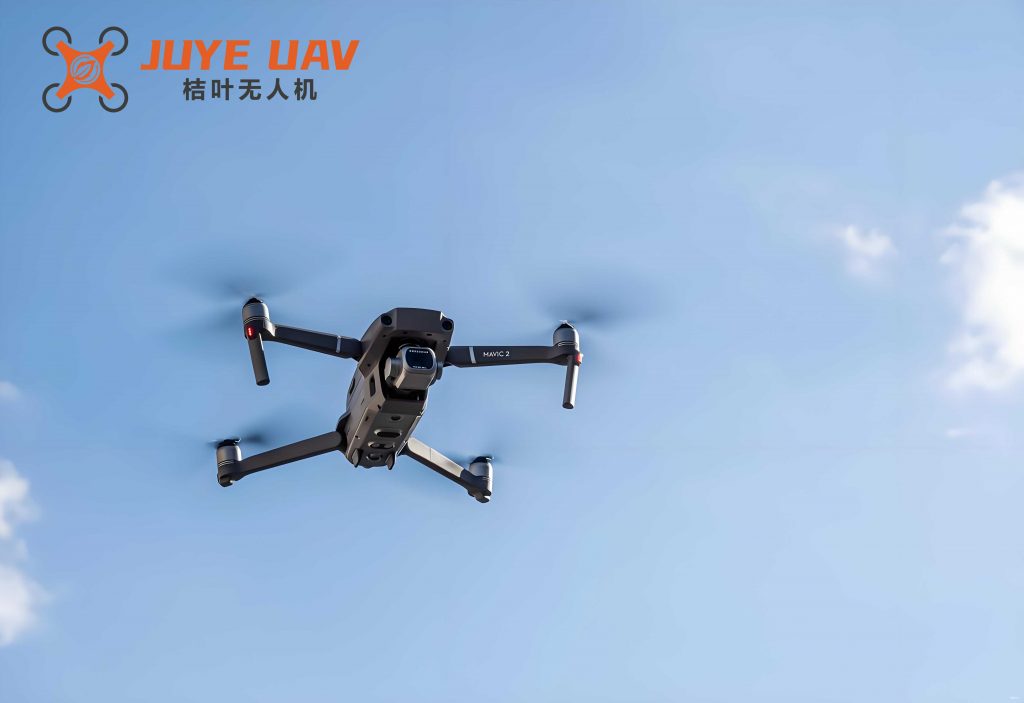
A quadrotor drone is an underactuated system with six degrees of freedom (position $$[x, y, z]$$ and orientation $$[\phi, \theta, \psi]$$) but only four independent control inputs (the rotational speeds of its four motors, $$\omega_i$$). The “X” configuration is adopted for its enhanced stability compared to the “+” configuration. The control inputs are transformed into a total thrust force $$F_T$$ and three torques $$[\tau_\phi, \tau_\theta, \tau_\psi]$$ about the body-frame axes through the following mixing matrix:
$$
\begin{bmatrix} F_T \\ \tau_\phi \\ \tau_\theta \\ \tau_\psi \end{bmatrix} =
\begin{bmatrix}
k_F & k_F & k_F & k_F \\
0 & -k_F l & 0 & k_F l \\
-k_F l & 0 & k_F l & 0 \\
k_M & -k_M & k_M & -k_M
\end{bmatrix}
\begin{bmatrix} \omega_1^2 \\ \omega_2^2 \\ \omega_3^2 \\ \omega_4^2 \end{bmatrix}
$$
where $$k_F$$ is the thrust coefficient, $$k_M$$ is the moment (drag) coefficient, and $$l$$ is the arm length from the center of mass to each motor. The squared terms reflect the relationship between propeller speed and thrust/torque. The attitude dynamics, relating torques to angular acceleration, are given by the Euler rotation equations:
$$
\boldsymbol{\tau} = \mathbf{I} \dot{\boldsymbol{\omega}} + \boldsymbol{\omega} \times (\mathbf{I} \boldsymbol{\omega})
$$
where $$\boldsymbol{\tau} = [\tau_\phi, \tau_\theta, \tau_\psi]^T$$ is the torque vector, $$\mathbf{I}$$ is the inertia matrix of the quadrotor drone, and $$\boldsymbol{\omega} = [p, q, r]^T$$ is the body-frame angular velocity vector.
1.2 Digital Twin Construction in Gazebo
To enable effective DRL training, we constructed a high-fidelity digital twin within the Gazebo simulator. This process involved several key steps:
1.2.1 3D Geometry and Inertial Properties: A simplified yet physically accurate 3D model of the quadrotor drone was created, comprising the frame, four motors, propellers, battery, and flight controller. The mass $$m$$ of each component was measured, and assuming uniform density, the volume $$V$$ and inertia tensor $$\mathbf{I’}$$ were computed from the mesh. The final inertia $$\mathbf{I}$$ was scaled using the formula:
$$
\mathbf{I} = \mathbf{I’} \cdot \text{unit\_scale}^2 \cdot \frac{m}{V}
$$
where `unit_scale` converts from modeling units to meters. Component masses are summarized in the table below.
| Component | Mass (g) |
|---|---|
| Battery | 184.2 |
| Frame | 82.0 |
| Motor (each) | 33.0 |
| Propeller (each) | 5.3 |
| Flight Controller Assembly | 106.0 |
1.2.2 Inertial Measurement Unit (IMU) Model: Real-world sensor noise is critical for sim-to-real transfer. We characterized the noise of the on-board gyroscope by collecting data from a stationary quadrotor drone. The noise for each axis was found to approximate a Gaussian distribution. The measured parameters are shown below.
| Axis | Mean $$\mu$$ (deg/s) | Std. Dev. $$\sigma$$ (deg/s) |
|---|---|---|
| Roll ($$\phi$$) | -0.071 | 0.14 |
| Pitch ($$\theta$$) | 0.64 | 0.14 |
| Yaw ($$\psi$$) | 0.29 | 0.13 |
These noise profiles were injected into the simulated IMU readings within Gazebo.
1.2.3 Propulsion System Model: The motor-propeller dynamics were modeled using blade element theory. Thrust $$T$$ and torque $$Q$$ are proportional to the square of the rotational speed $$\omega$$:
$$
T(\omega) = k_T \omega^2, \quad Q(\omega) = k_Q \omega^2
$$
The coefficients $$k_T$$ and $$k_Q$$ were determined experimentally on a test stand by measuring maximum thrust, torque, and RPM. Using standard aerodynamic relations involving thrust coefficient $$C_T$$, torque coefficient $$C_Q$$, air density $$\rho$$, and propeller diameter $$D$$:
$$
k_T = \frac{C_T \rho D^4}{(2\pi)^2}, \quad k_Q = \frac{C_Q \rho D^5}{(2\pi)^2}
$$
we derived the final coefficients used in our simulation, characterizing the propulsion system of our specific quadrotor drone.
| Parameter | Value |
|---|---|
| $$k_T$$ | $$1.920 \times 10^{-6}$$ N/RPM² |
| $$k_Q$$ | $$1.781 \times 10^{-7}$$ Nm/RPM² |
| Max Thrust per Motor | 5.39 N |
2. Deep Reinforcement Learning for Attitude Control
We frame the problem of angular rate control for the quadrotor drone as a sequential decision-making task solvable via DRL. The core is the formulation of a Markov Decision Process (MDP).
2.1 Markov Decision Process Formulation
An MDP is defined by the tuple $$(\mathcal{S}, \mathcal{A}, \mathcal{P}, \mathcal{R}, \gamma)$$: state space, action space, state transition probability, reward function, and discount factor.
2.1.1 State Space $$\mathcal{S}$$: The state should provide the agent with sufficient information to make a control decision. We define the state at time $$t$$ as a 6-dimensional vector:
$$
\mathbf{s}_t = [\mathbf{e}_t, \Delta\mathbf{e}_t]
$$
where $$\mathbf{e}_t = \boldsymbol{\Omega}^*_t – \boldsymbol{\Omega}_t$$ is the angular rate error between the target $$\boldsymbol{\Omega}^*_t = [p^*, q^*, r^*]^T$$ and the measured rate $$\boldsymbol{\Omega}_t$$ from the IMU. $$\Delta\mathbf{e}_t = \mathbf{e}_t – \mathbf{e}_{t-1}$$ is the derivative of the error, providing information about the trend. This state representation is concise and provides the agent with both proportional and derivative information, analogous to a PD controller but to be processed by a neural network.
2.1.2 Action Space $$\mathcal{A}$$: The action is the direct command to the quadrotor drone’s actuators. We define the action $$\mathbf{a}_t$$ as a 4-dimensional vector in the range [0, 1], representing the normalized PWM command sent to each of the four Electronic Speed Controllers (ESCs). This maps directly to the motor thrusts $$[T_1, T_2, T_3, T_4]$$.
2.1.3 Reward Function $$\mathcal{R}$$: Designing an effective reward function is critical for guiding the learning process. Our reward at time $$t$$ is a composite function encouraging fast, accurate, and efficient tracking:
$$
r_t = r_{track} + r_{smooth} + r_{min\_cmd} + r_{overact} + r_{lazy}
$$
- Tracking Reward $$r_{track}$$: Penalizes the squared angular rate error.
$$ r_{track} = -\alpha_1 (e_\phi^2 + e_\theta^2 + e_\psi^2) $$ - Smoothing Reward $$r_{smooth}$$: Penalizes large changes in consecutive motor commands to reduce jitter and mechanical stress.
$$ r_{smooth} = -\alpha_2 \cdot \max(|\Delta \mathbf{y}_t|) $$ where $$\mathbf{y}_t$$ is the action vector. - Minimal Command Reward $$r_{min\_cmd}$$: Encourages using the minimum necessary control effort, saving energy.
$$ r_{min\_cmd} = \alpha_3 \cdot (1 – \bar{\mathbf{y}}_t) $$ where $$\bar{\mathbf{y}}_t$$ is the mean action. - Over-Actuation Penalty $$r_{overact}$$: Strongly penalizes if any motor command is saturated at 1.0 for extended periods, indicating loss of control authority.
$$ r_{overact} = -\alpha_4 \cdot \mathbb{I}(\exists y_i = 1.0) $$ - Lazy Policy Penalty $$r_{lazy}$$: Penalizes the agent if it outputs a near-zero command when a non-zero target is given, preventing it from learning a “do-nothing” policy.
$$ r_{lazy} = -\alpha_5 \cdot \mathbb{I}(\mathbf{y}_t \approx \mathbf{0} \land \boldsymbol{\Omega}^*_t \neq \mathbf{0}) $$
The coefficients $$\alpha_{1:5}$$ are hyperparameters tuned to balance these objectives.
2.2 Proximal Policy Optimization (PPO) Algorithm
We selected PPO as our training algorithm due to its stability, sample efficiency, and proven performance in continuous control tasks like operating a quadrotor drone. PPO is an actor-critic method that maintains two neural networks: a policy network (actor) $$\pi_\theta(\mathbf{a}|\mathbf{s})$$ parameterized by $$\theta$$, and a value network (critic) $$V_\phi(\mathbf{s})$$ parameterized by $$\phi$$.
The core objective of PPO is to maximize a surrogate loss function $$L^{CLIP}(\theta)$$ while preventing excessively large policy updates that can collapse performance. The clipped objective is:
$$
L^{CLIP}(\theta) = \hat{\mathbb{E}}_t \left[ \min\left( \rho_t(\theta) \hat{A}_t, \text{clip}(\rho_t(\theta), 1-\epsilon, 1+\epsilon) \hat{A}_t \right) \right]
$$
where $$\rho_t(\theta) = \frac{\pi_\theta(\mathbf{a}_t|\mathbf{s}_t)}{\pi_{\theta_{old}}(\mathbf{a}_t|\mathbf{s}_t)}$$ is the probability ratio between the new and old policies, $$\hat{A}_t$$ is an estimate of the advantage function (computed by the critic network using Generalized Advantage Estimation), and $$\epsilon$$ is a clipping hyperparameter (e.g., 0.2). The `clip` term modifies the surrogate objective by removing the incentive for moving $$\rho_t$$ outside the interval $$[1-\epsilon, 1+\epsilon]$$. This simple mechanism ensures stable and monotonic policy improvement. The value network is trained to minimize the mean-squared error against the estimated returns.
3. Training and Performance Evaluation
3.1 Experimental Setup and Baseline
Training was conducted in the Gazebo simulation interfaced with the GymFC framework. The PPO policy and value networks were simple Multi-Layer Perceptrons (MLPs) with two hidden layers. We trained for a total of $$10^7$$ timesteps. A well-tuned PID controller served as our primary baseline. Its parameters $$[K_P, K_I, K_D]$$ for each axis were carefully adjusted using industry-standard methods to represent a competent traditional controller for the quadrotor drone.
| PPO Hyperparameter | Value |
|---|---|
| Total Timesteps | $$10^7$$ |
| Learning Rate | $$3 \times 10^{-4}$$ |
| Horizon (T) | 2048 |
| Mini-batch Size | 64 |
| Clipping Parameter ($$\epsilon$$) | 0.2 |
| Discount Factor ($$\gamma$$) | 0.99 |
| GAE Parameter ($$\lambda$$) | 0.95 |
3.2 Training Analysis
The learning curve for the PPO controller showed stable and monotonic improvement, converging after approximately $$4 \times 10^6$$ timesteps to a high average reward. This indicates the agent successfully learned a policy that balances fast tracking with smooth, efficient control of the quadrotor drone. For comparison, we also trained a controller using the Soft Actor-Critic (SAC) algorithm. While SAC also converged, its training was less stable initially and its final performance, as shown in the evaluation, was inferior to PPO for this specific task.
3.3 Performance Comparison and Results
We evaluated the trained PPO controller against the PID baseline and the SAC controller using a series of challenging step-response tests on all three axes (roll, pitch, yaw). Key performance metrics were measured: Rise Time (time to go from 10% to 90% of the command), Settling Time (time to reach and stay within ±10% of the command), Overshoot (percentage of maximum peak exceeding the command), and Steady-State Error.
The quantitative results are compelling and are summarized in the tables below. First, a general tracking error analysis on random signals shows the fundamental improvement.
| Controller | Metric | Roll (p) | Pitch (q) | Yaw (r) | Average |
|---|---|---|---|---|---|
| PPO | MAE (deg/s) | 0.33 | 0.56 | 0.92 | 0.60 |
| MSE ((deg/s)²) | 2.11 | 9.05 | 18.69 | 9.95 | |
| PID | MAE (deg/s) | 7.08 | 4.71 | 7.58 | 6.46 |
| MSE ((deg/s)²) | 644.31 | 281.29 | 647.83 | 524.48 |
The PPO controller achieves an order-of-magnitude lower Mean Squared Error (MSE), indicating vastly superior tracking precision for the quadrotor drone. The step-response metrics tell a similar story of superior agility and stability.
| Performance Metric | PPO (Avg) | PID (Avg) | Improvement |
|---|---|---|---|
| Rise Time (ms) | 38.7 | 86.7 | 55.4% Faster |
| Settling Time (ms) | 78.0 | 180.0 | 56.7% Faster |
| Overshoot (%) | 33.1 | 63.4 | 47.8% Less |
| Steady-State Error (%) | 0.72 | 0.73 | Comparable |
The PPO-based quadrotor drone controller demonstrates a dramatic improvement in dynamic response. It reacts to command changes more than twice as quickly (55.4% faster rise time) and achieves a stable state in less than half the time (56.7% faster settling time). Crucially, it accomplishes this with significantly less overshoot (47.8% reduction), meaning it approaches the desired attitude more directly and with less oscillation. The steady-state error, where PID controllers traditionally excel, is matched by the learned controller. The SAC controller, while functional, exhibited longer rise/settling times and higher steady-state error than both PPO and PID.
4. Conclusion and Future Work
In this work, we have successfully developed and validated a high-performance attitude controller for a quadrotor drone using Deep Reinforcement Learning. By constructing a high-fidelity simulation model and formulating the angular rate control problem as an MDP, we trained a neural network policy using the PPO algorithm. The learned controller fundamentally addresses key limitations of conventional PID control: it eliminates the need for manual parameter tuning and demonstrates objectively superior performance in terms of response speed and stability.
Our simulation experiments provide strong evidence that the DRL-based controller for the quadrotor drone achieves significantly faster rise and settling times—key metrics for agile flight—while simultaneously reducing overshoot by nearly half. This translates to a more responsive, stable, and predictable aircraft, which is essential for executing complex maneuvers or operating in turbulent conditions.
This research establishes a solid foundation for intelligent flight control. Future work will focus on several important avenues. Firstly, investigating sim-to-real transfer is paramount; techniques like domain randomization and adaptive control will be employed to bridge the gap between simulation and physical quadrotor drone tests. Secondly, we plan to extend the control hierarchy by using this low-rate controller as a stable inner loop for training a high-level position or trajectory tracking controller also using DRL. Finally, exploring on-line adaptation mechanisms will allow the quadrotor drone to continuously fine-tune its policy in response to changing dynamics, such as payload variations or component wear, pushing the boundaries towards fully autonomous and resilient aerial systems.