
The trajectory tracking problem for unmanned aerial vehicles (UAVs), particularly quadrotor drones, has garnered immense research interest due to their versatile applications in surveillance, inspection, search and rescue, and payload delivery. The intrinsic characteristics of a quadrotor drone, such as vertical take-off and landing (VTOL), hovering capability, and agile maneuverability, make it an ideal platform for these tasks. However, its dynamical model is inherently nonlinear, underactuated, and strongly coupled. Furthermore, during flight operations, a quadrotor drone is invariably subject to external disturbances like wind gusts and parametric uncertainties. These factors pose significant challenges in designing a control system that guarantees precise and stable trajectory tracking amidst such complexities.
In this comprehensive analysis, we delve into the design of a robust trajectory tracking controller for a quadrotor drone. The primary objective is to force the drone’s position $\mathbf{p} = [x, y, z]^T$ and attitude to accurately follow a predefined, time-varying desired trajectory $\mathbf{p}_d(t)$, even in the presence of bounded external disturbances. The core of our approach lies in the synergistic application of the Sliding Mode Control (SMC) methodology and the Unit Quaternion for attitude representation. SMC is renowned for its robustness against matched uncertainties and disturbances, while unit quaternions provide a globally non-singular parameterization of the drone’s orientation, effectively avoiding the well-known “gimbal lock” problem associated with Euler angles. We will systematically develop the dynamical model, design the control laws using a combination of backstepping and sliding mode techniques, and validate the controller’s performance through numerical simulations.
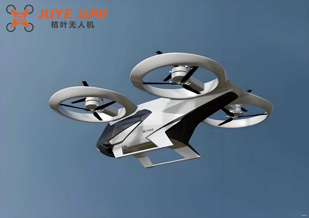
The standard dynamic model of a quadrotor drone is derived using the Newton-Euler formalism. We define two coordinate frames: the inertial frame $\mathcal{I} = \{ \mathbf{i}_x, \mathbf{i}_y, \mathbf{i}_z \}$ and the body-fixed frame $\mathcal{B} = \{ \mathbf{b}_x, \mathbf{b}_y, \mathbf{b}_z \}$ attached to the drone’s center of mass. The translational dynamics are governed by the forces acting on the vehicle, while the rotational dynamics describe the evolution of its attitude.
The complete dynamics can be separated into translational (position) and rotational (attitude) subsystems:
1. Translational Dynamics:
$$ m \ddot{\mathbf{p}} = -R(\mathbf{Q}) u_1 \mathbf{e}_3 + m g \mathbf{e}_3 + \boldsymbol{\delta}_F $$
where $m$ is the mass, $g$ is the gravitational acceleration, $\mathbf{e}_3 = [0, 0, 1]^T$, $u_1$ is the total thrust input (control input), $R(\mathbf{Q})$ is the rotation matrix from $\mathcal{B}$ to $\mathcal{I}$ expressed using the unit quaternion $\mathbf{Q}$, and $\boldsymbol{\delta}_F$ represents bounded external disturbance forces acting on the quadrotor drone, satisfying $|\boldsymbol{\delta}_F| \leq D_F$.
2. Rotational Dynamics (using Unit Quaternion):
The attitude is represented by a unit quaternion $\mathbf{Q} = [\boldsymbol{\eta}^T, q]^T = [q_1, q_2, q_3, q]^T$, satisfying $\boldsymbol{\eta}^T \boldsymbol{\eta} + q^2 = 1$. The kinematics and dynamics are:
$$ \dot{\mathbf{Q}} = \frac{1}{2} \begin{pmatrix} q \mathbf{I}_3 + \boldsymbol{\eta}^\times \\ -\boldsymbol{\eta}^T \end{pmatrix} \boldsymbol{\Omega} $$
$$ J \dot{\boldsymbol{\Omega}} = \boldsymbol{\tau} – \boldsymbol{\Omega}^\times J \boldsymbol{\Omega} + \boldsymbol{\delta}_{\tau} $$
where $\boldsymbol{\Omega} = [p, q, r]^T$ is the angular velocity vector in $\mathcal{B}$, $J = \text{diag}(I_{xx}, I_{yy}, I_{zz})$ is the inertia matrix, $\boldsymbol{\tau}$ is the control torque input vector, $\boldsymbol{\delta}_{\tau}$ is the bounded external disturbance torque ($|\boldsymbol{\delta}_{\tau}| \leq D_{\tau}$), and $(\cdot)^\times$ denotes the skew-symmetric matrix operator.
The rotation matrix in terms of the unit quaternion is given by:
$$ R(\mathbf{Q}) = (q^2 – \boldsymbol{\eta}^T \boldsymbol{\eta}) \mathbf{I}_3 + 2 \boldsymbol{\eta} \boldsymbol{\eta}^T – 2 q \boldsymbol{\eta}^\times $$
This representation is crucial for avoiding singularities when the quadrotor drone performs aggressive maneuvers.
The control problem is underactuated: we have four control inputs ($u_1$ and $\boldsymbol{\tau}$) but six degrees of freedom to track (position and attitude). The standard approach is hierarchical: design a controller for the translational subsystem that outputs a desired attitude and the total thrust $u_1$, and then design a controller for the rotational subsystem to track this desired attitude. We employ a Sliding Mode Control strategy for both layers to ensure robustness.
Step 1: Position Tracking Controller Design
We define the position error $\mathbf{e}_p = \mathbf{p} – \mathbf{p}_d$. The translational dynamics can be rewritten by introducing an intermediate virtual control input $\mathbf{F} = [F_1, F_2, F_3]^T = m R(\mathbf{Q}_d) \mathbf{e}_3 u_1$, where $\mathbf{Q}_d$ is the desired quaternion. This allows us to partially decouple the position control from the specific attitude. The dynamics become:
$$ m \ddot{\mathbf{p}} = m g \mathbf{e}_3 – \mathbf{F} – u_1 \mathbf{A} \boldsymbol{\eta}_e + \boldsymbol{\delta}_F $$
where $\boldsymbol{\eta}_e$ is the vector part of the attitude error quaternion and $\mathbf{A}$ is a matrix derived from the quaternion error. The term $- u_1 \mathbf{A} \boldsymbol{\eta}_e$ acts as a coupling disturbance from the attitude tracking error.
We now design $\mathbf{F}$ using a robust backstepping sliding mode approach. Let $\mathbf{v} = \dot{\mathbf{p}}$ and define the first error variable $\mathbf{z}_1 = \mathbf{e}_p$. Define a first sliding surface:
$$ \mathbf{s}_1 = \dot{\mathbf{z}}_1 + k_1 \mathbf{z}_1 = \mathbf{v} – \dot{\mathbf{p}}_d + k_1 \mathbf{e}_p $$
where $k_1 > 0$ is a constant gain. Consider the Lyapunov function candidate $V_1 = \frac{1}{2} \mathbf{s}_1^T \mathbf{s}_1$. Its derivative is:
$$ \dot{V}_1 = \mathbf{s}_1^T \dot{\mathbf{s}}_1 = \mathbf{s}_1^T (\dot{\mathbf{v}} – \ddot{\mathbf{p}}_d + k_1 \dot{\mathbf{e}}_p) $$
Substituting the dynamics $\dot{\mathbf{v}} = g \mathbf{e}_3 – \frac{1}{m}\mathbf{F} – \frac{u_1}{m} \mathbf{A} \boldsymbol{\eta}_e + \frac{1}{m}\boldsymbol{\delta}_F$ yields:
$$ \dot{V}_1 = \mathbf{s}_1^T \left( g \mathbf{e}_3 – \frac{1}{m}\mathbf{F} – \frac{u_1}{m} \mathbf{A} \boldsymbol{\eta}_e + \frac{1}{m}\boldsymbol{\delta}_F – \ddot{\mathbf{p}}_d + k_1 (\mathbf{v} – \dot{\mathbf{p}}_d) \right) $$
We choose the virtual control law $\mathbf{F}$ as:
$$ \mathbf{F} = m \left[ g \mathbf{e}_3 – \ddot{\mathbf{p}}_d + k_1 (\mathbf{v} – \dot{\mathbf{p}}_d) + k_2 \mathbf{s}_1 + \rho_1 \frac{\mathbf{s}_1}{||\mathbf{s}_1|| + \epsilon_1} \right] $$
where $k_2 > 0$, $\rho_1 \geq D_F$ is a robust gain to counteract the disturbance $\boldsymbol{\delta}_F$, and $\epsilon_1$ is a small smoothing constant to alleviate chattering. The term involving $\mathbf{A} \boldsymbol{\eta}_e$ is treated as a bounded disturbance due to the subsequent attitude controller’s action. With this choice, the derivative becomes:
$$ \dot{V}_1 \leq -k_2 ||\mathbf{s}_1||^2 + \mathbf{s}_1^T \left( \frac{\boldsymbol{\delta}_F}{m} – \rho_1 \frac{\mathbf{s}_1}{||\mathbf{s}_1|| + \epsilon_1} \right) – \frac{u_1}{m} \mathbf{s}_1^T \mathbf{A} \boldsymbol{\eta}_e $$
Using the property $\mathbf{s}_1^T \boldsymbol{\delta}_F \leq ||\mathbf{s}_1|| D_F$, it can be shown that $\dot{V}_1$ is negative definite outside a small boundary layer, ensuring the sliding surface $\mathbf{s}_1$ is attractive. Consequently, the position tracking error $\mathbf{e}_p$ converges to a small neighborhood of zero.
From the calculated $\mathbf{F}$, we can extract the desired total thrust $u_1$ and the desired attitude $\mathbf{Q}_d$. The desired thrust magnitude is simply the norm of the projection:
$$ u_1 = ||\mathbf{F}|| $$
The desired body $z$-axis direction (in $\mathcal{I}$) is given by $\mathbf{z}_{B,d} = \mathbf{F} / ||\mathbf{F}||$. Combined with a desired yaw angle $\psi_d(t)$, we can construct the full desired rotation matrix $R_d$ and then convert it to the desired unit quaternion $\mathbf{Q}_d$.
Step 2: Attitude Tracking Controller Design
The objective is to drive the actual quaternion $\mathbf{Q}$ to the desired quaternion $\mathbf{Q}_d$. Define the error quaternion $\tilde{\mathbf{Q}} = \tilde{[}\boldsymbol{\eta}_e^T, q_e]^T = \mathbf{Q}_d^{-1} \otimes \mathbf{Q}$. The corresponding error dynamics are:
$$ \dot{\tilde{\mathbf{Q}}} = \frac{1}{2} \begin{pmatrix} q_e \mathbf{I}_3 + \boldsymbol{\eta}_e^\times \\ -\boldsymbol{\eta}_e^T \end{pmatrix} \tilde{\boldsymbol{\Omega}} $$
$$ J \dot{\tilde{\boldsymbol{\Omega}}} = \boldsymbol{\tau} – \boldsymbol{\Omega}^\times J \boldsymbol{\Omega} + \boldsymbol{\delta}_{\tau} – J( \dot{\boldsymbol{\Omega}}_d – \tilde{\boldsymbol{\Omega}}^\times R(\tilde{\mathbf{Q}}) \boldsymbol{\Omega}_d ) $$
where $\tilde{\boldsymbol{\Omega}} = \boldsymbol{\Omega} – R(\tilde{\mathbf{Q}}) \boldsymbol{\Omega}_d$ is the angular velocity error and $\boldsymbol{\Omega}_d$ is the desired angular velocity derived from $\mathbf{Q}_d$.
We design the control torque $\boldsymbol{\tau}$ directly using a sliding mode approach. Define the second sliding surface for the attitude:
$$ \mathbf{s}_2 = \tilde{\boldsymbol{\Omega}} + \Lambda \boldsymbol{\eta}_e $$
where $\Lambda = \text{diag}(\lambda_1, \lambda_2, \lambda_3)$, $\lambda_i > 0$. This surface combines angular velocity and orientation error. Consider the Lyapunov function $V_2 = \frac{1}{2} \mathbf{s}_2^T J \mathbf{s}_2 + 2k_q (1 – q_e)$, where $k_q > 0$. The term $2(1 – q_e)$ is positive definite with respect to the attitude error. The derivative is:
$$ \dot{V}_2 = \mathbf{s}_2^T J \dot{\mathbf{s}}_2 – k_q \boldsymbol{\eta}_e^T \tilde{\boldsymbol{\Omega}} $$
Substituting the error dynamics and after considerable algebraic manipulation, we choose the control law:
$$ \boldsymbol{\tau} = \boldsymbol{\Omega}^\times J \boldsymbol{\Omega} + J( \dot{\boldsymbol{\Omega}}_d – \tilde{\boldsymbol{\Omega}}^\times R(\tilde{\mathbf{Q}}) \boldsymbol{\Omega}_d ) – J \Lambda \dot{\boldsymbol{\eta}}_e – K_{\Omega} \mathbf{s}_2 – \rho_2 \frac{\mathbf{s}_2}{||\mathbf{s}_2|| + \epsilon_2} + k_q J \boldsymbol{\eta}_e $$
where $K_{\Omega} > 0$ is a positive definite gain matrix, $\rho_2 \geq D_{\tau}$ is the robust gain against disturbance torque, and $\epsilon_2$ is a smoothing constant. This control law leads to:
$$ \dot{V}_2 \leq -\mathbf{s}_2^T K_{\Omega} \mathbf{s}_2 + \mathbf{s}_2^T \boldsymbol{\delta}_{\tau} – \rho_2 \frac{\mathbf{s}_2^T \mathbf{s}_2}{||\mathbf{s}_2|| + \epsilon_2} $$
Again, using the disturbance bound, $\dot{V}_2$ can be made negative definite, forcing $\mathbf{s}_2 \to 0$. On the sliding manifold $\mathbf{s}_2 = 0$, we have $\tilde{\boldsymbol{\Omega}} = -\Lambda \boldsymbol{\eta}_e$, which leads to the reduced-order attitude error dynamics $\dot{\boldsymbol{\eta}}_e = \frac{1}{2}(q_e \mathbf{I}_3 + \boldsymbol{\eta}_e^\times)(-\Lambda \boldsymbol{\eta}_e)$. This system is asymptotically stable, guaranteeing that $\boldsymbol{\eta}_e \to 0$ and consequently $q_e \to \pm 1$. The desired equilibrium $q_e = 1$ (zero rotation error) can be made globally asymptotically stable with proper initialization or an additional term in the control law.
The following table summarizes the key parameters used for the quadrotor drone model in the subsequent simulation:
| Parameter | Symbol | Value |
|---|---|---|
| Mass | $m$ | 3.0 kg |
| Gravity | $g$ | 9.81 m/s² |
| Inertia (xx) | $I_{xx}$ | 0.039 kg·m² |
| Inertia (yy) | $I_{yy}$ | 0.039 kg·m² |
| Inertia (zz) | $I_{zz}$ | 0.039 kg·m² |
To validate the proposed robust sliding mode controller, numerical simulations are performed in a MATLAB/Simulink environment. The desired trajectory for the quadrotor drone is a 3D Lissajous-like curve:
$$ \mathbf{p}_d(t) = \begin{bmatrix} 0.5 \sin(\frac{\pi t}{5}) \\ 2.5 \sin(\frac{\pi t}{5}) \\ 0.5t \end{bmatrix} \text{m} $$
This trajectory commands motion along all three axes. The initial position of the drone is set to $[0, 0, 0]^T$ with an initial attitude error.
Disturbances: To test robustness, significant time-varying disturbances are injected:
$$ \boldsymbol{\delta}_F(t) = \begin{bmatrix} 0.1\sin(0.1\pi t) \\ 0.2\sin(0.1\pi t) \\ 0.3\sin(0.2\pi t) \end{bmatrix} \text{N}, \quad \boldsymbol{\delta}_{\tau}(t) = \begin{bmatrix} 0.1\sin(0.1\pi t) \\ 0.2\cos(0.1\pi t) \\ 0.3\sin(0.2\pi t) \end{bmatrix} \text{N·m} $$
The bounds are $D_F = 1$ N and $D_{\tau} = 1$ N·m. The controller gains are tuned as follows:
| Gain | Symbol | Value |
|---|---|---|
| Position sliding gain 1 | $k_1$ | 2.0 |
| Position sliding gain 2 | $k_2$ | 5.0 |
| Position robust gain | $\rho_1$ | 5.0 |
| Attitude sliding gain | $\Lambda$ | 10 $\mathbf{I}_3$ |
| Attitude damping gain | $K_{\Omega}$ | 15 $\mathbf{I}_3$ |
| Attitude robust gain | $\rho_2$ | 15.0 |
| Quaternion error gain | $k_q$ | 15.0 |
Simulation Results:
1. Trajectory Tracking: The quadrotor drone accurately tracks the desired 3D path. The position errors $\mathbf{e}_p$ converge to a very small neighborhood of zero (on the order of $10^{-3}$ m) within approximately 2-3 seconds, despite the persistent disturbances. This demonstrates the effectiveness and robustness of the position control loop.
2. Attitude Tracking: The vector part of the quaternion error $\boldsymbol{\eta}_e$ converges rapidly to near zero within about 1 second. The scalar part $q_e$ converges to 1, indicating that the actual attitude successfully aligns with the desired attitude computed by the position controller. This fast and stable convergence is critical for maintaining the accuracy of the position tracking loop.
3. Control Inputs: The generated control inputs—the total thrust $u_1$ and the three control torques $\boldsymbol{\tau}$—are smooth and bounded. The sliding mode action is evident in high-frequency switching at the beginning to reject initial errors and disturbances, which is then smoothed by the boundary layer parameters ($\epsilon_1, \epsilon_2$) to produce practically implementable signals. The thrust $u_1$ varies smoothly to accommodate the changing demands of the trajectory against gravity and disturbances.
The simulation confirms that the integrated control strategy successfully manages the coupling between translation and rotation. The position controller generates a feasible attitude command, and the robust attitude controller tracks it precisely, thereby enabling accurate trajectory tracking for the overall quadrotor drone system.
This study has presented a comprehensive robust control solution for the trajectory tracking problem of a quadrotor drone. The key contributions are the integration of unit quaternions to avoid kinematic singularities and the application of sliding mode control to ensure robustness against external disturbances. The control structure is hierarchical yet coupled through the desired attitude generation. The position controller, designed via a robust backstepping sliding mode approach, ensures convergence of the tracking error. The attitude controller, a direct sliding mode controller on a combined sliding surface, provides fast and accurate orientation tracking. The stability of the entire closed-loop system was rigorously analyzed using Lyapunov theory.
The proposed method effectively addresses major challenges in controlling a quadrotor drone: underactuation, strong nonlinear coupling, and external disturbances. The simulation results under significant time-varying disturbances validate the theoretical design, showing rapid convergence, high tracking accuracy, and smooth, bounded control inputs. Future work may involve extending this framework to address actuator saturation, model parameter uncertainties through adaptive techniques, and experimental validation on a physical quadrotor drone platform.