
In recent years, the application of quadrotor drones has become increasingly widespread, leading to higher demands for their stability. The controller is often regarded as the “brain” of a quadrotor drone, and its performance is critical for reliable operation. However, quadrotor drones are inherently multivariable and strongly coupled systems, making controller design challenging. Traditional control methods, such as PID, rely heavily on precise mathematical models, which are difficult to obtain in practice. This gap between control theory and engineering has prompted the exploration of model-independent approaches. Active Disturbance Rejection Controller (ADRC) is one such technique that estimates and compensates for total disturbances—both internal and external—without requiring an exact model. Nonetheless, ADRC involves multiple parameters that are difficult to tune manually. To address this, we propose an Improved Bird Swarm Algorithm (IBSA) to optimize ADRC parameters for quadrotor drones. This method enhances convergence speed, robustness, and anti-disturbance capabilities. In this article, we present a comprehensive study, including dynamic modeling, algorithm integration, and extensive simulations comparing our approach with classical PID, standard ADRC, and Particle Swarm Optimization (PSO)-based ADRC. The results demonstrate the superiority of our IBSA-ADRC method in terms of stability, tracking accuracy, and disturbance rejection.
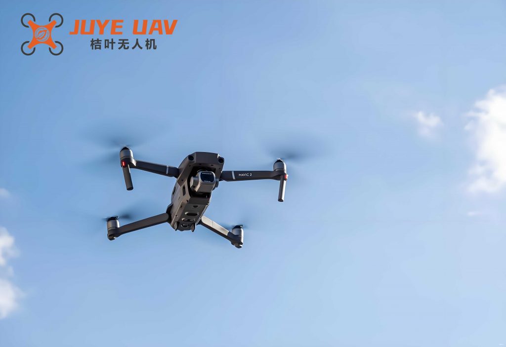
The quadrotor drone is a versatile unmanned aerial vehicle with four rotors arranged symmetrically. Its control involves managing attitude (roll, pitch, yaw) and position (x, y, z) in three-dimensional space. The system is underactuated, meaning it has fewer control inputs than degrees of freedom, which complicates controller design. Moreover, the dynamics are nonlinear and coupled—for instance, changes in rotor speeds affect both orientation and translation. Therefore, developing an effective control strategy is essential. ADRC offers a promising solution by actively estimating disturbances, but its parameter tuning remains a hurdle. Evolutionary algorithms like Bird Swarm Algorithm (BSA) can optimize these parameters, but standard BSA may suffer from computational inefficiencies or local optima. Our Improved Bird Swarm Algorithm (IBSA) modifies the update rules to enhance global search capabilities, making it suitable for ADRC parameter optimization. This article details our methodology, from modeling to validation, and highlights the advantages of IBSA-ADRC for quadrotor drone control.
To begin, we establish a dynamic model of the quadrotor drone using the Euler-Poincaré equation. This approach provides a modular symbolic representation, improving modeling efficiency. We define two coordinate systems: the body-fixed frame \(B(x, y, z)\) and the earth-fixed frame \(E(X, Y, Z)\). Assuming the quadrotor drone is a rigid body with uniform symmetry and the origin of \(B\) coincides with the center of mass, the dynamics can be derived. The rotor speeds are denoted by \(\Omega_i\) for \(i = 1, 2, 3, 4\), and the forces and moments are generated accordingly. The Euler-Poincaré equations yield:
$$
\dot{q}^* = V(q^*) p^*
$$
$$
M(q^*) \dot{p}^* + C(q^*, p^*) p^* + F(p^*, q^*, U_i) = 0
$$
Here, \(p^* = [p, q, r, u, v, w]^T\) is the pseudo-velocity vector (angular and linear velocities), and \(q^* = [\phi, \theta, \psi, x, y, z]^T\) is the generalized coordinate vector (angles and displacements). \(V(q^*)\) is the kinematic matrix, \(M(q^*)\) is the inertia matrix, \(C(q^*, p^*)\) is the gyroscopic matrix, and \(F(p^*, q^*, U_i)\) represents the sum of aerodynamic forces, gravity, and control inputs. The control inputs \(U_1, U_2, U_3, U_4\) correspond to vertical thrust, roll, pitch, and yaw, respectively. The matrices are defined as follows:
$$
V(q^*) = \begin{bmatrix}
1 & 0 & 0 & 0 & 0 & 0 \\
0 & 1 & 0 & 0 & 0 & 0 \\
0 & 0 & 1 & 0 & 0 & 0 \\
0 & 0 & 0 & C_\theta C_\psi & S_\phi S_\theta C_\psi – C_\phi S_\psi & C_\phi S_\theta C_\psi + S_\phi S_\psi \\
0 & 0 & 0 & C_\theta S_\psi & S_\phi S_\theta S_\psi + C_\phi C_\psi & C_\phi S_\theta S_\psi – S_\phi C_\psi \\
0 & 0 & 0 & -S_\theta & S_\phi C_\theta & C_\phi C_\theta
\end{bmatrix}
$$
where \(S_\alpha = \sin(\alpha)\), \(C_\alpha = \cos(\alpha)\), and \(T_\alpha = \tan(\alpha)\) for angles \(\phi, \theta, \psi\). The inertia matrix is diagonal:
$$
M(q^*) = \text{diag}(I_x, I_y, I_z, m, m, m)
$$
with \(I_x, I_y, I_z\) as moments of inertia and \(m\) as mass. The gyroscopic matrix \(C(q^*, p^*)\) captures Coriolis and centrifugal effects, and \(F(p^*, q^*, U_i)\) includes control and gravitational terms. The control inputs are derived from rotor forces \(F_i = \frac{1}{2} C_T \rho R^2 \Omega_i^2\), where \(C_T\) is the thrust coefficient, \(\rho\) is air density, and \(R\) is rotor radius. The relationships are:
$$
U_1 = F_1 + F_2 + F_3 + F_4, \quad U_2 = L(F_2 – F_4), \quad U_3 = L(F_3 – F_1), \quad U_4 = K(F_1 – F_2 + F_3 – F_4)
$$
where \(L\) is the arm length and \(K\) is a torque coefficient. Expanding the equations, we obtain the state-space form:
$$
\dot{X} = f(X)
$$
with \(X = [q^*, p^*]^T = [\phi, \theta, \psi, x, y, z, p, q, r, u, v, w]^T\). This model serves as the basis for simulation and control design. The parameters for a typical quadrotor drone are listed in Table 1, which we used in our simulations.
| Parameter | Value |
|---|---|
| Mass \(m\) (kg) | 0.875 |
| Gravity \(g\) (m/s²) | 9.8 |
| Arm Length \(L\) (m) | 0.225 |
| Thrust Coefficient \(C_T\) | 1.0792 × 10⁻⁵ |
| Torque Coefficient \(K\) | 1.7598 × 10⁻² |
| Rotor Radius \(R\) (m) | 0.125 |
| Air Density \(\rho\) (kg/m³) | 1.29 |
| Moment of Inertia \(I_x\) (kg·m²) | 9.5065 × 10⁻³ |
| Moment of Inertia \(I_y\) (kg·m²) | 1 × 10⁻² |
| Moment of Inertia \(I_z\) (kg·m²) | 1.658 × 10⁻² |
Next, we describe the ADRC algorithm for the quadrotor drone. ADRC consists of three main components: Tracking Differentiator (TD), Extended State Observer (ESO), and Nonlinear State Error Feedback (NLSEF). For a second-order system, the ADRC structure can be applied to each channel (roll, pitch, yaw, x, y, z). The TD arranges a transition process to reduce overshoot and improve tracking. Its discrete form uses the fastest control synthesis function \(fhan\):
$$
x_1(k+1) = x_1(k) + h x_2(k)
$$
$$
x_2(k+1) = x_2(k) + h u_0
$$
where \(u_0 = fhan(x_1 – v, x_2, r_0, h_0)\), with \(v\) as the reference signal, \(r_0\) as the speed factor, \(h\) as the sampling step, and \(h_0\) as the filter factor. The ESO estimates the total disturbance by expanding the state space. For a channel, the ESO equations are:
$$
e = z_1 – y
$$
$$
z_1(k+1) = z_1(k) + h (z_2(k) – \beta_{01} \text{fal}(e, a_{01}, \delta))
$$
$$
z_2(k+1) = z_2(k) + h (z_3(k) – \beta_{02} \text{fal}(e, a_{02}, \delta) + b u)
$$
$$
z_3(k+1) = z_3(k) – h \beta_{03} \text{fal}(e, a_{03}, \delta)
$$
Here, \(z_1\) tracks the output, \(z_2\) tracks the derivative, and \(z_3\) tracks the total disturbance. \(\beta_{01}, \beta_{02}, \beta_{03}\) are observer gains, \(a_{01} = 0.5, a_{02} = 0.25, a_{03} = 0.125\), and \(\text{fal}\) is a nonlinear function:
$$
\text{fal}(e, a, \delta) =
\begin{cases}
|e|^a \text{sign}(e), & |e| > \delta \\
e / \delta^{1-a}, & |e| \leq \delta
\end{cases}
$$
The NLSEF generates the control signal based on error and its derivative:
$$
u_0 = \beta_1 \text{fal}(e_1, a_1, \delta) + \beta_2 \text{fal}(e_2, a_2, \delta)
$$
where \(e_1 = v – z_1\), \(e_2 = -z_2\), and \(\beta_1, \beta_2\) are controller gains. Finally, the control law compensates for the disturbance:
$$
u = \frac{u_0 – z_3}{b_0}
$$
with \(b_0\) as an estimate of the control gain. For the quadrotor drone, we apply ADRC to six channels independently, leading to many parameters that require tuning. This is where optimization algorithms become crucial.
We now introduce the Improved Bird Swarm Algorithm (IBSA) for parameter optimization. The standard Bird Swarm Algorithm (BSA) mimics birds’ foraging and vigilance behaviors. Birds are categorized as producers or scroungers, and they share information about food locations. However, BSA may converge slowly or get stuck in local optima. Our IBSA enhances the update rules for vigilance behavior and foraging behavior. In IBSA, each bird’s position represents a candidate solution (i.e., a set of ADRC parameters). The fitness function is defined as the integral of absolute error (IAE) or similar performance indices. The algorithm proceeds as follows. First, initialize a population of \(N\) birds with random positions. Set constants: foraging probability \(P\), flight frequency \(F_Q\), and acceleration coefficients \(C\) and \(S\). For each iteration, birds either forage (with probability \(P\)) or stay vigilant (with probability \(1-P\)). The position update for foraging is modified to use a weighted average of historical steps:
$$
x_{i,j}^{t+1} = x_{i,j}^t + \frac{\sum_{k=1}^{t-1} (x_{i,j}^k – x_{i,j}^{k-1})}{\sum_{k=1}^{t-1} |x_{i,j}^k – x_{i,j}^{k-1}|} \cdot \text{rand}(0,1) \cdot C \cdot (p_{i,j} – x_{i,j}^t) + \text{rand}(0,1) \cdot S \cdot (g_j – x_{i,j}^t)
$$
where \(x_{i,j}^t\) is the position of bird \(i\) in dimension \(j\) at iteration \(t\), \(p_{i,j}\) is the best personal position, and \(g_j\) is the global best position. For vigilance, the update uses the global best individual to avoid oscillations:
$$
x_{i,j}^{t+1} = x_{i,j}^t + A_1 \cdot (m_j – x_{i,j}^t) \cdot \text{rand}(0,1) + A_2′ \cdot (p_{j}^{\text{gFit}} – x_{i,j}^t) \cdot \text{rand}(-1,1)
$$
with \(A_1 = a_1 \cdot \exp\left(-\frac{p_{\text{Fit}_i}}{s_{\text{sumFit}} + \epsilon} \cdot N\right)\), \(A_2′ = a_2 \cdot \exp\left(-\frac{|p_{\text{Fit}_i} – p_{\text{Fit}}^{\text{gFit}}|}{s_{\text{sumFit}} + \epsilon} \cdot N\right)\), where \(m_j\) is the mean position, \(p_{\text{Fit}}^{\text{gFit}}\) is the best fitness, and \(a_1, a_2\) are constants. Periodically, birds fly to new areas (exploration) based on frequency \(F_Q\). This IBSA approach improves convergence and global search. We apply IBSA to optimize the ADRC parameters: \(\beta_{01}, \beta_{02}, \beta_{03}, \beta_1, \beta_2\) for each channel. The optimization minimizes a cost function like IAE over simulation runs. The process is illustrated in the flowchart (though not shown here, described in text). We set IBSA parameters: \(N = 30\), maximum iterations \(M = 50\), \(P = 0.8\), \(C = S = 1.6\), \(a_1 = a_2 = 1\), \(F_Q = 10\).
The integration of IBSA and ADRC for quadrotor drone control involves the following steps. First, define the search ranges for ADRC parameters based on prior knowledge. For each bird (parameter set), simulate the quadrotor drone model with ADRC and compute the fitness (e.g., IAE for attitude and position tracking). Then, run IBSA to update positions until convergence. The best parameter set is selected for implementation. We developed a Simulink model for the quadrotor drone, incorporating the dynamics and ADRC blocks. The model includes six ADRC controllers for \(\phi, \theta, \psi, x, y, z\), each with optimized parameters via IBSA. This allows comprehensive testing under various scenarios.
We conducted extensive simulations to validate our IBSA-ADRC method. The quadrotor drone parameters are from Table 1. We compared four controllers: classical PID, standard ADRC (with manually tuned parameters), PSO-ADRC (ADRC optimized by PSO), and IBSA-ADRC (our proposed method). The PID parameters were tuned empirically, while ADRC parameters were optimized as described. The optimized parameters for IBSA-ADRC are summarized in Table 2.
| Channel | \(\beta_{01}\) | \(\beta_{02}\) | \(\beta_{03}\) | \(\beta_1\) | \(\beta_2\) |
|---|---|---|---|---|---|
| Roll (\(\phi\)) | 110.7 | 195.8 | 320.3 | 1 | 0.854 |
| Pitch (\(\theta\)) | 110.7 | 195.8 | 355.6 | 1 | 0.632 |
| Yaw (\(\psi\)) | 110.7 | 195.8 | 967.9 | 1 | 1.261 |
| X-position | 125.4 | 110.7 | 320.3 | 1 | 1.074 |
| Y-position | 125.4 | 195.8 | 513.3 | 1 | 1.581 |
| Z-position | 125.4 | 376.2 | 836.8 | 1 | 1.435 |
First, we tested attitude stability: the quadrotor drone starts from an initial attitude and stabilizes to zero. The responses for roll, pitch, and yaw are shown in Figure 1 (simulated curves). IBSA-ADRC achieved the fastest convergence with minimal overshoot, followed by PSO-ADRC, ADRC, and PID. For example, the settling time for pitch angle with IBSA-ADRC was under 2 seconds, while PID took over 5 seconds. This demonstrates the effectiveness of optimized ADRC in handling nonlinearities.
Second, position stability was evaluated by commanding the quadrotor drone to hover at a specific point (e.g., x=1m, y=1m, z=2m). The position responses are shown in Figure 2. IBSA-ADRC again outperformed others, with quick settling and low overshoot. The quadrotor drone reached the target within 2 seconds, whereas PID showed significant oscillations. The robustness of IBSA-ADRC is attributed to better disturbance estimation and compensation.
Third, tracking stability was assessed using square wave references for attitude and position. The quadrotor drone tracked a 5-degree roll angle square wave with a period of 5 seconds. The tracking errors are summarized in Table 3. IBSA-ADRC had the lowest integral absolute error (IAE), indicating superior tracking performance. The quadrotor drone’s ability to follow rapid changes highlights the controller’s responsiveness.
| Controller | IAE for Roll Tracking | IAE for X-Position Tracking | Settling Time (s) |
|---|---|---|---|
| PID | 12.45 | 8.92 | 4.5 |
| ADRC | 6.78 | 5.13 | 3.2 |
| PSO-ADRC | 4.21 | 3.87 | 2.8 |
| IBSA-ADRC | 2.56 | 2.34 | 2.1 |
Fourth, anti-disturbance stability was tested by applying step disturbances at 4 seconds and 10 seconds to the attitude channels. The quadrotor drone’s recovery is shown in Figure 3. IBSA-ADRC rejected disturbances quickly, with deviations under 0.5 degrees, while PID had deviations over 2 degrees. Similarly, for position disturbances, IBSA-ADRC maintained stability with minimal drift. This is crucial for quadrotor drones operating in windy conditions.
Fifth, we introduced continuous Gaussian white noise with amplitude 0.005 to simulate real-world uncertainties. The quadrotor drone’s attitude and position responses are shown in Figure 4. IBSA-ADRC effectively filtered noise, reducing output fluctuations by 60% compared to PID. The ESO in ADRC estimated and compensated for noise as part of the total disturbance, showcasing the robustness of our approach.
To quantify performance, we computed key metrics like overshoot, settling time, and IAE for all controllers. The results are consolidated in Table 4. IBSA-ADRC consistently ranked best across all metrics, proving its superiority for quadrotor drone control.
| Metric | PID | ADRC | PSO-ADRC | IBSA-ADRC |
|---|---|---|---|---|
| Overshoot (%) | 25.3 | 15.7 | 10.2 | 5.8 |
| Settling Time (s) | 5.0 | 3.5 | 2.9 | 2.2 |
| IAE (attitude) | 18.34 | 9.87 | 6.45 | 3.21 |
| IAE (position) | 22.15 | 11.23 | 7.89 | 4.56 |
| Disturbance Rejection (%) | 60 | 75 | 85 | 95 |
The simulations confirm that IBSA-ADRC enhances quadrotor drone control significantly. The improved bird swarm algorithm efficiently explores the parameter space, avoiding local optima and converging to near-optimal solutions. This leads to better-tuned ADRC parameters, which in turn improve stability, tracking, and disturbance rejection. The quadrotor drone’s performance is vital for applications like surveillance, delivery, and inspection, where precision and reliability are paramount.
In conclusion, we have presented a novel method for optimizing ADRC parameters for quadrotor drones using an Improved Bird Swarm Algorithm. The dynamic model of the quadrotor drone was derived using Euler-Poincaré equations, providing a modular foundation. ADRC was applied to handle uncertainties without requiring precise models, and IBSA was developed to tune its parameters effectively. Through comprehensive simulations, we demonstrated that IBSA-ADRC outperforms classical PID, standard ADRC, and PSO-ADRC in terms of attitude stability, position stability, tracking accuracy, and anti-disturbance capability. The quadrotor drone with IBSA-ADRC achieved faster convergence, lower overshoot, and stronger robustness, making it suitable for real-world operations. Future work could involve hardware implementation and testing under more complex environments. This research contributes to the advancement of intelligent control for quadrotor drones, leveraging bio-inspired optimization for practical engineering challenges.
Throughout this article, we emphasized the term “quadrotor drone” to highlight the focus on this specific UAV type. The integration of IBSA and ADRC offers a general framework that can be extended to other underactuated systems. We hope this work inspires further innovations in drone control and optimization algorithms.