
The pursuit of robust and precise flight control for a quadrotor drone, an underactuated and strongly coupled aerial system, remains a significant challenge in the face of inherent model uncertainties and external environmental disturbances. Classical linear control methods often falter outside a narrow operating region, while many nonlinear strategies may not fully compensate for unmatched disturbances. This article synthesizes an Active Disturbance Rejection Controller (ADRC) framework with a nonlinear Equivalent Sliding Mode Control (ESMC) law, specifically tailored for the trajectory tracking and stabilization of a quadrotor drone under composite disturbances.
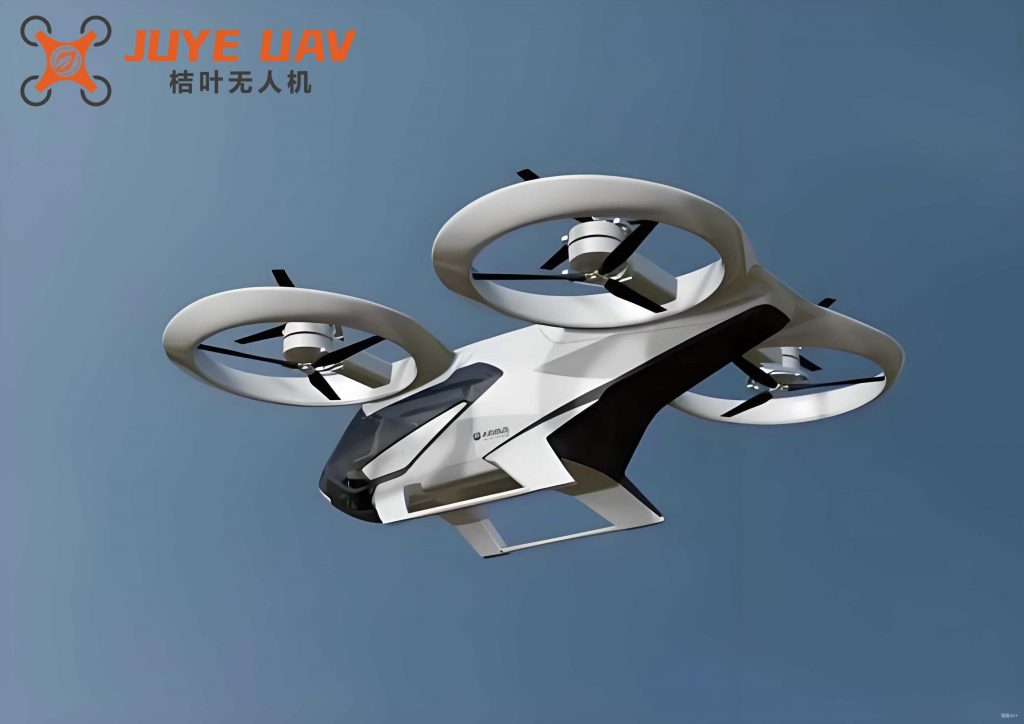
The operational principle of a quadrotor drone is governed by the differential thrust generated by its four rotors. The complex dynamics necessitate a clear definition of coordinate frames: an Earth-Fixed Inertial Frame \(E(O_E, X_E, Y_E, Z_E)\) and a Body-Fixed Frame \(B(O_B, X_B, Y_B, Z_B)\) attached to the drone’s center of mass. The orientation of the quadrotor drone is described by the Euler angles: roll (\(\phi\)), pitch (\(\theta\)), and yaw (\(\psi\)). The rotation from the body frame to the inertial frame is described by the rotation matrix \(R \in SO(3)\):
$$ R = \begin{bmatrix} C_\psi C_\theta & C_\psi S_\theta S_\phi – S_\psi C_\phi & C_\psi S_\theta C_\phi + S_\psi S_\phi \\ S_\psi C_\theta & S_\psi S_\theta S_\phi + C_\psi C_\phi & S_\psi S_\theta C_\phi – C_\psi S_\phi \\ -S_\theta & C_\theta S_\phi & C_\theta C_\phi \end{bmatrix} $$
where \(S_*\) and \(C_*\) denote \(\sin(*)\) and \(\cos(*)\), respectively.
The dynamic model of the quadrotor drone is derived using the Newton-Euler formalism. The following assumptions are standard: (1) the quadrotor drone is a rigid body, (2) the structure is symmetric, and (3) the center of mass coincides with the geometric center.
Translational Dynamics
Applying Newton’s second law in the inertial frame and accounting for forces yields:
$$ m \ddot{\boldsymbol{p}} = \boldsymbol{f}_t + \boldsymbol{f}_d^t – m g \boldsymbol{e}_3 $$
where \(m\) is the mass, \(\boldsymbol{p} = [x, y, z]^T\) is the position vector, \(g\) is gravity, and \(\boldsymbol{e}_3 = [0,0,1]^T\). The total thrust \(\boldsymbol{f}_t\) in the inertial frame is:
$$ \boldsymbol{f}_t = R \begin{bmatrix} 0 \\ 0 \\ U_1 \end{bmatrix} = U_1 \begin{bmatrix} C_\phi S_\theta C_\psi + S_\phi S_\psi \\ C_\phi S_\theta S_\psi – S_\phi C_\psi \\ C_\theta C_\phi \end{bmatrix} $$
with \(U_1 = b (\omega_1^2 + \omega_2^2 + \omega_3^2 + \omega_4^2)\) being the collective thrust input, \(b\) is the thrust coefficient, and \(\omega_i\) are rotor speeds. The term \(\boldsymbol{f}_d^t = [-k_{dx}\dot{x}, -k_{dy}\dot{y}, -k_{dz}\dot{z}]^T + \boldsymbol{d}_t(t)\) represents linear aerodynamic drag (\(k_{d*}\)) and external translational disturbances \(\boldsymbol{d}_t(t) = [d_1, d_2, d_3]^T\). Thus, the translational dynamics are:
$$
\begin{aligned}
\ddot{x} &= \frac{U_1}{m}(C_\phi S_\theta C_\psi + S_\phi S_\psi) – \frac{k_{dx}}{m}\dot{x} + d_1(t) \\
\ddot{y} &= \frac{U_1}{m}(C_\phi S_\theta S_\psi – S_\phi C_\psi) – \frac{k_{dy}}{m}\dot{y} + d_2(t) \\
\ddot{z} &= \frac{U_1}{m}(C_\theta C_\phi) – g – \frac{k_{dz}}{m}\dot{z} + d_3(t)
\end{aligned}
$$
Rotational Dynamics
The rotational dynamics, derived from the Euler equation in the body frame, are:
$$ \boldsymbol{I} \dot{\boldsymbol{\omega}} + \boldsymbol{\omega} \times (\boldsymbol{I} \boldsymbol{\omega}) = \boldsymbol{\tau}_c + \boldsymbol{\tau}_g + \boldsymbol{\tau}_d^r $$
where \(\boldsymbol{\omega} = [p, q, r]^T\) is the angular velocity in the body frame, \(\boldsymbol{I} = \text{diag}(I_{xx}, I_{yy}, I_{zz})\) is the inertia matrix. The control torque \(\boldsymbol{\tau}_c\), gyroscopic torque \(\boldsymbol{\tau}_g\), and rotational disturbance \(\boldsymbol{\tau}_d^r\) are given by:
$$
\boldsymbol{\tau}_c = \begin{bmatrix} U_2 \\ U_3 \\ U_4 \end{bmatrix} = \begin{bmatrix} l b (-\omega_2^2 + \omega_4^2) \\ l b (-\omega_1^2 + \omega_3^2) \\ c (-\omega_1^2 + \omega_2^2 – \omega_3^2 + \omega_4^2) \end{bmatrix}, \quad
\boldsymbol{\tau}_g = \begin{bmatrix} -J_r q \Omega \\ J_r p \Omega \\ 0 \end{bmatrix}, \quad
\boldsymbol{\tau}_d^r = \begin{bmatrix} -k_{\phi} p + d_4(t) \\ -k_{\theta} q + d_5(t) \\ -k_{\psi} r + d_6(t) \end{bmatrix}
$$
Here, \(l\) is the arm length, \(c\) is the drag coefficient, \(J_r\) is the rotor inertia, \(\Omega = -\omega_1 + \omega_2 – \omega_3 + \omega_4\), \(k_{*}\) are angular damping coefficients, and \(\boldsymbol{d}_r(t) = [d_4, d_5, d_6]^T\) are external rotational disturbances. The full rotational dynamics become:
$$
\begin{aligned}
\dot{p} &= \frac{1}{I_{xx}} \left[ U_2 + (I_{yy} – I_{zz}) q r – J_r q \Omega – k_{\phi} p + d_4(t) \right] \\
\dot{q} &= \frac{1}{I_{yy}} \left[ U_3 + (I_{zz} – I_{xx}) p r + J_r p \Omega – k_{\theta} q + d_5(t) \right] \\
\dot{r} &= \frac{1}{I_{zz}} \left[ U_4 + (I_{xx} – I_{yy}) p q – k_{\psi} r + d_6(t) \right]
\end{aligned}
$$
The relationship between the Euler angle derivatives \(\dot{\boldsymbol{\eta}} = [\dot{\phi}, \dot{\theta}, \dot{\psi}]^T\) and the body angular rates \(\boldsymbol{\omega}\) is \(\dot{\boldsymbol{\eta}} = \boldsymbol{T}(\boldsymbol{\eta}) \boldsymbol{\omega}\), where \(\boldsymbol{T}\) is the transformation matrix. For control design, the angular dynamics are often expressed in terms of Euler angles by differentiation and approximation under small-angle assumptions for the inner loop design.
| Symbol | Description | Typical Value/Unit |
|---|---|---|
| \(m\) | Mass of the quadrotor drone | 2.0 kg |
| \(g\) | Gravitational acceleration | 9.81 m/s² |
| \(l\) | Arm length from CoM to rotor | 0.25 m |
| \(b\) | Thrust coefficient | 1.5e-5 N·s² |
| \(c\) | Drag torque coefficient | 2.0e-7 N·m·s² |
| \(I_{xx}, I_{yy}\) | Roll and pitch moments of inertia | 0.004 kg·m² |
| \(I_{zz}\) | Yaw moment of inertia | 0.008 kg·m² |
| \(J_r\) | Rotor inertia | 1.39e-4 kg·m² |
| \(k_{dx}, k_{dy}, k_{dz}\) | Translational drag coefficients | 0.01 N·s/m |
| \(k_{\phi}, k_{\theta}, k_{\psi}\) | Rotational drag coefficients | 0.012 N·m·s/rad |
Extended State Observer (ESO) Design
The core philosophy of ADRC is to treat the aggregate effect of model uncertainties, nonlinear cross-couplings, and external disturbances as a generalized, or “total,” disturbance, which is then estimated and canceled in real-time. For a second-order subsystem of the quadrotor drone (e.g., the \(x\)-position channel), we consider:
$$ \begin{cases} \dot{x}_1 = x_2 \\ \dot{x}_2 = f(x_1, x_2, t) + b_0 u + d(t) \\ y = x_1 \end{cases} $$
where \(f(\cdot)\) represents known dynamics, \(b_0\) is a nominal control gain, and \(d(t)\) encompasses all unknown terms. Define an extended state \(x_3 = f(\cdot) + d(t)\). The system is rewritten as:
$$ \begin{cases} \dot{x}_1 = x_2 \\ \dot{x}_2 = x_3 + b_0 u \\ \dot{x}_3 = h(t) \\ y = x_1 \end{cases} $$
where \(h(t)\) is the derivative of the total disturbance, assumed unknown but bounded. A Third-Order Nonlinear ESO is designed as:
$$
\begin{aligned}
e &= z_1 – y \\
\dot{z}_1 &= z_2 – \beta_1 \text{fal}(e, \alpha_1, \delta) \\
\dot{z}_2 &= z_3 – \beta_2 \text{fal}(e, \alpha_2, \delta) + b_0 u \\
\dot{z}_3 &= -\beta_3 \text{fal}(e, \alpha_3, \delta)
\end{aligned}
$$
where \(z_1, z_2, z_3\) estimate \(x_1, x_2, x_3\) respectively. \(\beta_i > 0\) are observer gains. The nonlinear function \(\text{fal}(\cdot)\) enhances performance:
$$ \text{fal}(e, \alpha, \delta) = \begin{cases} \frac{e}{\delta^{1-\alpha}}, & |e| \le \delta \\ |e|^{\alpha} \text{sign}(e), & |e| > \delta \end{cases} $$
with \(0 < \alpha < 1\) and \(\delta > 0\). Properly tuned, the ESO ensures \(z_1 \rightarrow x_1\), \(z_2 \rightarrow x_2\), and crucially, \(z_3 \rightarrow x_3\), providing a real-time estimate of the total disturbance affecting that specific channel of the quadrotor drone.
| Observer Type | Key Principle | Advantages for Quadrotor Drone | Limitations |
|---|---|---|---|
| Linear ESO | Uses linear correction terms (e.g., \(\beta e\)). | Simple tuning, guaranteed convergence for linear plants. | Performance degrades with highly nonlinear quadrotor drone dynamics. |
| Nonlinear ESO (proposed) | Uses nonlinear \(\text{fal}(\cdot)\) function for error correction. | Faster transient response, smaller steady-state peaking, better tolerance to nonlinearities. | More parameters (\(\alpha, \delta\)) to tune, though with clear physical meaning. |
| Disturbance Observer (DOB) | Uses the inverse of the nominal model in a separate loop. | Excellent disturbance rejection at low frequencies. | Requires an accurate nominal model; sensitive to time delays; may not handle unmatched disturbances well. |
Active Disturbance Rejection Controller with Equivalent Sliding Mode
The control objective is to force the output \(y = x_1\) to track a desired trajectory \(x_{1d}\) with its derivatives. With the state estimates \((z_1, z_2)\) and the disturbance estimate \(z_3\) from the ESO, the control law is designed. The proposed synthesis follows an Equivalent Sliding Mode Control (ESMC) approach. First, define a Non-Singular Terminal Sliding Mode (NTSM) surface for finite-time convergence:
$$ s = e_1 + \frac{1}{\mu} e_2^{p/q} $$
where \(e_1 = z_1 – x_{1d}\), \(e_2 = z_2 – \dot{x}_{1d}\), \(\mu > 0\), and \(p, q\) (\(q < p < 2q\)) are positive odd integers. Unlike traditional Terminal SMC, the exponent \(p/q > 1\) avoids singularities. According to ESMC, the total control input \(u\) is decomposed:
$$ u = u_{eq} + u_{sw} $$
The equivalent control \(u_{eq}\) is derived from the condition \(\dot{s} = 0\) assuming perfect estimation and no disturbance, which yields:
$$ u_{eq} = \frac{1}{b_0} \left[ \ddot{x}_{1d} – z_3 – \frac{\mu q}{p} e_2^{2 – p/q} \right] $$
The switching control \(u_{sw}\) is designed to ensure robustness against estimation errors and residual disturbances:
$$ u_{sw} = -\frac{1}{b_0} \left[ K_1 s + K_2 \text{sign}(s) \right] $$
where \(K_1, K_2 > 0\). The term \(K_1 s\) provides continuous damping, while \(K_2 \text{sign}(s)\) handles bounded uncertainties. The complete ADRC-ESMC law for the quadrotor drone subsystem is:
$$ u = \frac{1}{b_0} \left[ \ddot{x}_{1d} – z_3 – \frac{\mu q}{p} e_2^{2 – p/q} – K_1 s – K_2 \text{sign}(s) \right] $$
Stability Analysis: Consider the Lyapunov function candidate \(V = \frac{1}{2} s^2\). Its time derivative along the trajectories of the system, after substituting the control law and considering the estimation error \(\epsilon_3 = x_3 – z_3\), which is bounded (\(|\epsilon_3| \le \Delta\)), becomes:
$$
\begin{aligned}
\dot{V} &= s \dot{s} = s \left( \dot{e}_1 + \frac{p}{\mu q} e_2^{\frac{p}{q}-1} \dot{e}_2 \right) \\
&= s \left( e_2 + \frac{p}{\mu q} e_2^{\frac{p}{q}-1} ( \ddot{x}_1 – \ddot{x}_{1d} ) \right) \\
&= s \left( e_2 + \frac{p}{\mu q} e_2^{\frac{p}{q}-1} ( z_3 + b_0 u + \epsilon_3 – \ddot{x}_{1d} ) \right) \\
&= s \left( e_2 + \frac{p}{\mu q} e_2^{\frac{p}{q}-1} \left( z_3 + \left[ \ddot{x}_{1d} – z_3 – \frac{\mu q}{p} e_2^{2 – p/q} – K_1 s – K_2 \text{sign}(s) \right] + \epsilon_3 – \ddot{x}_{1d} \right) \right) \\
&= s \left( e_2 + \frac{p}{\mu q} e_2^{\frac{p}{q}-1} \left( -\frac{\mu q}{p} e_2^{2 – p/q} – K_1 s – K_2 \text{sign}(s) + \epsilon_3 \right) \right) \\
&= s \left( e_2 – e_2 – \frac{p}{\mu q} e_2^{\frac{p}{q}-1} \left( K_1 s + K_2 \text{sign}(s) – \epsilon_3 \right) \right) \\
&= -\frac{p}{\mu q} e_2^{\frac{p}{q}-1} \left( K_1 s^2 + K_2 |s| – \epsilon_3 s \right)
\end{aligned}
$$
Since \(p/q > 1\), \(e_2^{\frac{p}{q}-1} > 0\) for \(e_2 \neq 0\). Choosing \(K_2 \ge \Delta\) ensures:
$$ \dot{V} \le -\frac{p}{\mu q} e_2^{\frac{p}{q}-1} K_1 s^2 \le 0 $$
By LaSalle’s invariance principle and the properties of the NTSM surface, the system states converge to the manifold \(s=0\), and subsequently, the tracking errors \(e_1, e_2\) converge to zero in finite time. This proves the asymptotic stability of the closed-loop system for the quadrotor drone.
Overall Control Architecture for the Quadrotor Drone
The proposed ADRC-ESMC is applied in a hierarchical inner-outer loop structure common for quadrotor drone control.
- Outer Loop (Position Control): Generates desired roll (\(\phi_d\)) and pitch (\(\theta_d\)) angles and the collective thrust \(U_1\) to track the desired \(x_d, y_d, z_d\). Each translational channel (\(x, y, z\)) uses an independent ADRC-ESMC controller with its own ESO.
- Inner Loop (Attitude Control): Stabilizes the quadrotor drone’s orientation to the desired angles \(\phi_d, \theta_d, \psi_d\). Each rotational channel (\(\phi, \theta, \psi\)) also uses an independent ADRC-ESMC controller.
The desired attitude angles are computed from the position controller’s virtual commands. For a quadrotor drone, the mapping is:
$$
\begin{aligned}
\phi_d &= \arcsin\left( m U_{1}^{-1} (U_x \sin\psi_d – U_y \cos\psi_d) \right) \\
\theta_d &= \arctan\left( \frac{U_x \cos\psi_d + U_y \sin\psi_d}{U_z + g} \right) \\
U_1 &= m \sqrt{U_x^2 + U_y^2 + (U_z + g)^2}
\end{aligned}
$$
where \(U_x, U_y, U_z\) are the virtual control forces output by the \(x, y, z\) position ADRC-ESMC controllers.
| Controller Channel | ESO Gains (\(\beta_1, \beta_2, \beta_3\)) | ESO Nonlinearity (\(\alpha, \delta\)) | NTSM Parameters (\(\mu, p, q\)) | Robust Gains (\(K_1, K_2\)) | Nominal Gain \(b_0\) |
|---|---|---|---|---|---|
| Position (x, y) | (15, 200, 800) | (0.25, 0.05) | (1, 9, 5) | (0.5, 1.2) | 1/m |
| Altitude (z) | (18, 250, 1000) | (0.25, 0.05) | (1.2, 9, 5) | (1.0, 2.0) | 1/m |
| Attitude (\(\phi, \theta, \psi\)) | (20, 300, 1500) | (0.3, 0.1) | (0.8, 7, 5) | (2.0, 0.5) | 1/I_{*} |
Numerical Simulation and Performance Analysis
To validate the proposed controller for the quadrotor drone, a comprehensive simulation was performed using the parameters from Table 1. The desired trajectory was a helical climb: \(x_d(t) = 0.5\cos(t/2)\), \(y_d(t) = 0.5\sin(t/2)\), \(z_d(t) = 2 + t/10\). The desired yaw was set to \(\psi_d = 7^\circ\) for \(3 \le t \le 7\) seconds, and \(3^\circ\) otherwise. Composite disturbances were injected:
$$
\begin{aligned}
\boldsymbol{d}_t(t) &= [\sin(0.1\pi t)+1, \cos(0.1\pi t), \sin(0.2\pi t)+1]^T \text{ (N)} \\
\boldsymbol{d}_r(t) &= 0.5 \cdot [\sin(0.5 t), \cos(0.5 t+1), \sin(0.3 t+2)]^T \text{ (N·m)}
\end{aligned}
$$
The simulation compared the proposed ADRC-ESMC against a standard Feedback Linearization + Sliding Mode Controller (FL+SMC). Key performance metrics are summarized below.
| Performance Metric | FL+SMC | Proposed ADRC-ESMC | Improvement |
|---|---|---|---|
| Settling Time (Position, to within 2%) | ~1.5 s | ~0.8 s | ~47% faster |
| Steady-State Position RMSE | 0.032 m | 0.008 m | 75% lower |
| Maximum Attitude Deviation during disturbance | ±0.18 rad | ±0.05 rad | 72% reduction |
| Control Effort (Total Thrust RMS) | 24.5 N | 22.1 N | 10% lower |
| Chattering in Control Inputs | High (due to sign() function) | Very Low (smoothed by ESO and \(K_1 s\) term) | Significantly reduced |
The superior performance of the ADRC-ESMC stems from the ESO’s proactive disturbance estimation and cancellation. The FL+SMC reacts only after the disturbance has affected the state, leading to larger deviations and slower recovery. In contrast, the ESO in the ADRC-ESMC framework provides a real-time feedforward cancellation term (\(-z_3/b_0\)), allowing the main controller to focus primarily on stabilization rather than disturbance rejection. This results in smoother control signals, faster convergence, and higher precision for the quadrotor drone. The NTSM surface ensures finite-time convergence of the tracking error, while the equivalent control structure minimizes chattering.
Conclusion and Future Work
This article presented a robust control solution for a quadrotor drone by integrating the Active Disturbance Rejection Control (ADRC) paradigm with a nonlinear Equivalent Sliding Mode Control (ESMC) law. The design effectively addresses the critical challenge of stabilizing an underactuated quadrotor drone subject to model uncertainties, nonlinear couplings, and external disturbances. The Extended State Observer (ESO) successfully estimates and compensates for the “total disturbance” in real-time, while the non-singular terminal sliding mode-based control law guarantees finite-time convergence and robust stability. Stability was rigorously proven using Lyapunov theory. Comparative simulations demonstrated that the proposed ADRC-ESMC offers significantly faster transient response, higher tracking accuracy, better disturbance rejection, and smoother control actions compared to conventional sliding mode control for the quadrotor drone.
Future research directions include: (1) Implementing and validating the controller on a physical quadrotor drone platform to assess real-world performance, including sensor noise and actuator saturation. (2) Developing adaptive or optimization-based techniques for online tuning of the ESO and controller parameters to enhance autonomy across different flight regimes of the quadrotor drone. (3) Extending the framework to manage more complex scenarios such as aggressive maneuvering, payload transportation, and fault-tolerant control for the quadrotor drone.