In recent years, the application of agricultural UAVs in plant protection has experienced explosive growth in China. As a researcher deeply involved in this field, I have witnessed and contributed to the evolution of these systems. Our company, focusing on innovation, has identified several limitations in commercially available agricultural UAVs, such as limited payload, lack of intelligent obstacle avoidance, and inefficiencies in terrain adaptation. To address these, we embarked on a comprehensive research and development program aimed at creating an agricultural UAV that excels in autonomous obstacle circumvention, terrain following, increased payload capacity, and operational efficiency. This article delves into our work, presenting technical insights, mathematical models, and practical applications that underscore the transformative potential of advanced agricultural UAVs.
The core of our agricultural UAV design revolves around four integrated systems: the flight control system, power system, communication link system, and spraying system. A modular architecture was adopted, allowing for rapid maintenance and component replacement, which is crucial for field operations. The airframe is constructed from lightweight composite materials, optimizing the strength-to-weight ratio. The propulsion system consists of brushless DC motors paired with electronic speed controllers (ESCs) and high-efficiency propellers. The thrust generated by each motor can be described by the standard propeller thrust equation:
$$ T = C_T \cdot \rho \cdot n^2 \cdot D^4 $$
where \( T \) is the thrust (in Newtons), \( C_T \) is the thrust coefficient, \( \rho \) is the air density (in kg/m³), \( n \) is the rotational speed (in revolutions per second), and \( D \) is the propeller diameter (in meters). For our agricultural UAV, we optimized \( C_T \) and \( D \) to achieve a lift-to-weight ratio exceeding 2.5, ensuring stable flight even with a full payload.
The flight controller is the brain of the agricultural UAV. We developed a custom industrial-grade flight control unit (FCU) running a real-time operating system. It processes data from an inertial measurement unit (IMU), global navigation satellite system (GNSS), and the DBF imaging radar to execute precise flight maneuvers. The control algorithm is based on a proportional-integral-derivative (PID) controller with adaptive tuning. The attitude control law for the roll axis, for instance, is given by:
$$ \delta_a = K_{p,\phi} \cdot e_\phi + K_{i,\phi} \cdot \int e_\phi \, dt + K_{d,\phi} \cdot \frac{de_\phi}{dt} $$
Here, \( \delta_a \) is the aileron control output, \( e_\phi = \phi_{desired} – \phi_{actual} \) is the roll angle error, and \( K_p, K_i, K_d \) are the tuned gains. Similar equations govern pitch and yaw. This ensures the agricultural UAV maintains stability against wind gusts and during aggressive maneuvering.
A pivotal innovation in our agricultural UAV is the DBF (Digital Beam Forming) imaging radar. Traditional ultrasonic or infrared sensors are often hampered by dust, light conditions, or limited range. Our radar operates in the millimeter-wave spectrum, providing high-resolution 3D point cloud data of the environment. The fundamental radar range equation, modified for a DBF phased array, helps understand its capability:
$$ P_r = \frac{P_t G_t G_r \lambda^2 \sigma}{(4\pi)^3 R^4 L} \cdot N_{elem} $$
where \( P_r \) is the received power, \( P_t \) is the transmitted power, \( G_t \) and \( G_r \) are the transmit and receive gains, \( \lambda \) is the wavelength, \( \sigma \) is the radar cross-section of the target, \( R \) is the range to the target, \( L \) is system loss, and \( N_{elem} \) is the number of array elements enhancing gain via beamforming. This allows our agricultural UAV to detect obstacles like trees or poles up to 30 meters away with centimeter-level accuracy.
The terrain-following function is critical for uniform chemical application on undulating fields. The radar continuously measures the distance to the crop canopy below the agricultural UAV. A control loop adjusts the UAV’s altitude \( h \) to maintain a constant setpoint \( h_{set} \). The algorithm can be expressed as:
$$ \dot{h}_{cmd} = K_{h} (h_{set} – h_{radar}) + K_{ff} \cdot \dot{S}_{terrain} $$
Here, \( \dot{h}_{cmd} \) is the commanded vertical velocity, \( K_h \) is a proportional gain, and \( K_{ff} \) is a feedforward gain that anticipates terrain slope \( \dot{S}_{terrain} \) derived from the radar’s forward scan. This enables the agricultural UAV to mimic the ground profile within a ±2 meter range, ensuring consistent spray deposition.
For autonomous obstacle circumvention, the DBF radar generates a real-time 3D occupancy grid. When an obstacle is detected within the flight path, the path planning module, based on an A* search algorithm, calculates an alternative trajectory. The cost function \( f(n) \) for the A* algorithm is:
$$ f(n) = g(n) + h(n) $$
where \( g(n) \) is the cost from the start node to node \( n \), and \( h(n) \) is a heuristic estimate of the cost from \( n \) to the goal. For our agricultural UAV, \( g(n) \) incorporates factors like energy consumption and turning radius, while \( h(n) \) is the Euclidean distance. This allows the agricultural UAV to smoothly deviate from the planned route and rejoin it post-obstacle, all without operator intervention.
The spraying system is another area of intensive research for our agricultural UAV. We moved away from traditional low-pressure nozzles to a high-pressure centrifugal atomization system. The Sauter Mean Diameter (SMD) of the droplets, a key metric for coverage and drift, is governed by:
$$ D_{32} = k \cdot \left( \frac{\mu}{\rho_l \omega^2 r} \right)^{0.6} \cdot \left( \frac{\sigma}{\rho_l \omega^2 r} \right)^{0.2} $$
In this equation, \( D_{32} \) is the SMD, \( k \) is a constant, \( \mu \) is the dynamic viscosity of the liquid, \( \rho_l \) is the liquid density, \( \omega \) is the angular velocity of the atomizer disc, \( r \) is the disc radius, and \( \sigma \) is the surface tension. By precisely controlling the motor driving the atomizer disc (and thus \( \omega \)), our agricultural UAV can produce droplet spectra ranging from 80 to 300 microns, optimizing for different agrochemicals and weather conditions to minimize drift.
The flow rate \( Q \) from the pump is regulated to match the agricultural UAV’s ground speed \( v \) and desired application rate \( AR \) (in liters per hectare):
$$ Q = \frac{AR \cdot v \cdot W}{600} $$
where \( W \) is the effective swath width (in meters). A flow meter provides closed-loop feedback to maintain \( Q \) within 2% of the target. This precision ensures chemical savings and environmental protection.
To address the payload limitation, we redesigned the liquid tank. Using finite element analysis (FEA), we optimized the tank geometry to maximize volume while minimizing weight and ensuring structural integrity during dynamic flight loads. The tank is made from food-grade polyethylene and features a quick-disconnect coupling system. The time \( t_{change} \) to swap an empty tank for a full one is now under 15 seconds, drastically improving operational tempo. The following table compares key parameters of our latest agricultural UAV (Model T16) with two previous generations and a competitor’s model.
| Model / Parameter | Our T16 | Our MG-1P | Competitor Alpha | Industry Avg. |
|---|---|---|---|---|
| Tank Capacity (L) | 16 | 10 | 12 | 10-12 |
| Max Takeoff Weight (kg) | 46.2 | 32.5 | 38.0 | ~35 |
| Operational Efficiency (ha/hr) | 10.0 | 6.0 | 7.5 | 6-7 |
| Battery Capacity (Wh) | 17,400 | 12,000 | 14,500 | ~13,000 |
| Spray System Pressure (MPa) | 0.8 | 0.3 | 0.5 | 0.3-0.5 |
| Obstacle Detection Range (m) | 30 | 10 (Ultrasonic) | 15 (Stereo Vision) | < 20 |
The operational efficiency \( \eta_{op} \) of an agricultural UAV can be modeled as a function of several variables:
$$ \eta_{op} = \frac{V_{tank} \cdot \rho_{liquid}}{t_{flight} + t_{turnaround}} \cdot \frac{1}{AR} \cdot C_{coverage} $$
where \( V_{tank} \) is tank capacity, \( \rho_{liquid} \) is liquid density, \( t_{flight} \) is flight time per sortie, \( t_{turnaround} \) is time for landing, refilling, and takeoff, \( AR \) is the application rate, and \( C_{coverage} \) is a coverage efficiency factor (typically 0.85-0.95). Our design improvements, particularly the larger tank and quick-swap system, significantly reduce \( t_{turnaround} \), boosting \( \eta_{op} \).
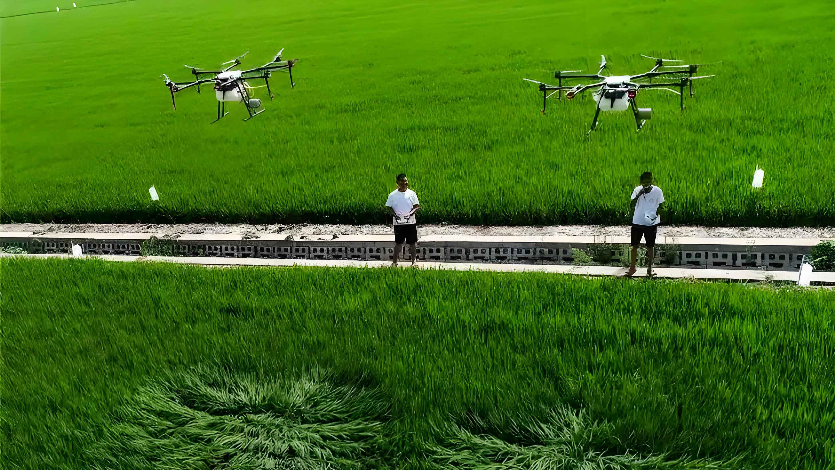
Field applications of our advanced agricultural UAV were conducted extensively in the rice-growing regions of Northeast China. The primary goals were to validate the autonomous obstacle avoidance in complex environments (featuring scattered trees, power lines, and farm structures) and to measure the improvement in spraying uniformity on sloped terrain. We set up multiple test plots with varying slopes and obstacle densities. The performance was quantified using water-sensitive papers placed at different canopy levels to analyze droplet deposition density \( N_d \) (droplets per cm²) and coverage percentage.
The deposition data was analyzed statistically. For a target \( N_d \) of 20 droplets/cm², our agricultural UAV achieved a coefficient of variation (CV) of less than 15% on flat terrain and below 25% on slopes up to 15 degrees, outperforming conventional systems whose CV often exceeds 40% on slopes. The CV is calculated as:
$$ CV = \frac{\sigma_{N_d}}{\mu_{N_d}} \times 100\% $$
where \( \sigma_{N_d} \) and \( \mu_{N_d} \) are the standard deviation and mean of droplet density across sampling points. The following table summarizes key results from one representative trial cycle.
| Trial Parameter | Flat Paddy Field | Sloped Field (10°) | Field with Dense Obstacles |
|---|---|---|---|
| Area Covered per Sortie (ha) | 1.2 | 1.1 | 1.0 |
| Avg. Droplet Density (droplets/cm²) | 22.5 | 19.8 | 21.3 |
| Coefficient of Variation (CV%) | 12.7 | 23.1 | 18.4 |
| Obstacle Avoidance Success Rate | N/A | N/A | 99.2% |
| Chemical Savings vs. Ground Rig | ~30% | ~25% | ~28% |
| Effective Field Capacity (ha/hr) | 9.8 | 9.0 | 8.5 |
The communication system employs an OcuSync digital link, providing a stable, low-latency connection up to a 3 km radius in open terrain. The link budget equation ensures reliable control and telemetry:
$$ P_{r,RC} = P_t + G_t + G_r – L_{path} – L_{fade} $$
where \( P_{r,RC} \) is received power at the remote controller, \( P_t \) is transmit power from the agricultural UAV, \( G_t \) and \( G_r \) are antenna gains, \( L_{path} \) is free-space path loss (\( 20\log_{10}(d) + 20\log_{10}(f) + 32.44 \), with \( d \) in km and \( f \) in MHz), and \( L_{fade} \) is the fade margin. This robust link allows the operator to monitor first-person view (FPV) video and all telemetry data, enabling pre-emptive decision-making.
Looking forward, the integration of artificial intelligence (AI) will be a game-changer for agricultural UAVs. We are developing machine learning models that can analyze multispectral imagery captured by the UAV in real-time to identify pest hotspots, nutrient deficiencies, or disease outbreaks. A convolutional neural network (CNN) for disease detection, for example, might process an image tensor \( I \in \mathbb{R}^{H \times W \times C} \) and output a probability map. The training minimizes a loss function such as categorical cross-entropy:
$$ \mathcal{L} = -\sum_{c=1}^{M} y_{o,c} \log(p_{o,c}) $$
where \( M \) is the number of disease classes, \( y \) is the binary indicator for the correct class, and \( p \) is the predicted probability. Such an AI agent on an agricultural UAV could prescribe variable-rate application maps on the fly, moving beyond uniform spraying to true precision agriculture.
Battery technology remains a critical constraint. The flight endurance \( T \) of an electric agricultural UAV is approximated by:
$$ T = \frac{E_{batt} \cdot \eta_{sys}}{P_{avg}} $$
where \( E_{batt} \) is the battery energy, \( \eta_{sys} \) is the total system efficiency (from battery to propeller thrust), and \( P_{avg} \) is the average power draw during mission. Current lithium-polymer batteries offer specific energies around 250 Wh/kg. We are actively researching hybrid power systems and rapid charging solutions to push \( T \) beyond 30 minutes for heavy-lift agricultural UAVs.
Furthermore, the concept of swarm operations using multiple coordinated agricultural UAVs is on the horizon. This involves distributed control algorithms where a fleet of \( N \) UAVs collaborates to cover a field. The total coverage time \( T_{swarm} \) can be modeled as:
$$ T_{swarm} \approx \frac{A_{field}}{N \cdot v \cdot W} + t_{sync} $$
where \( A_{field} \) is the field area, \( v \) is speed, \( W \) is individual swath width, and \( t_{sync} \) is the synchronization overhead. With an efficient communication mesh network, \( t_{sync} \) becomes negligible, promising linear scalability in productivity.
In conclusion, our research and development efforts have yielded an agricultural UAV that significantly advances the state of the art in autonomous operation, payload capacity, and spraying precision. The integration of DBF imaging radar for terrain following and obstacle circumvention, coupled with a high-efficiency centrifugal spraying system and a robust modular design, addresses the key pain points identified in earlier generations. Field trials confirm substantial gains in operational efficiency and chemical utilization. As we continue to innovate, focusing on AI-driven analytics, next-generation energy sources, and swarm intelligence, the agricultural UAV is poised to become an indispensable tool in the global pursuit of sustainable, efficient, and precise agriculture. The journey of this agricultural UAV from a concept to a field-proven solution illustrates the powerful synergy between aerospace engineering and agronomic science.