
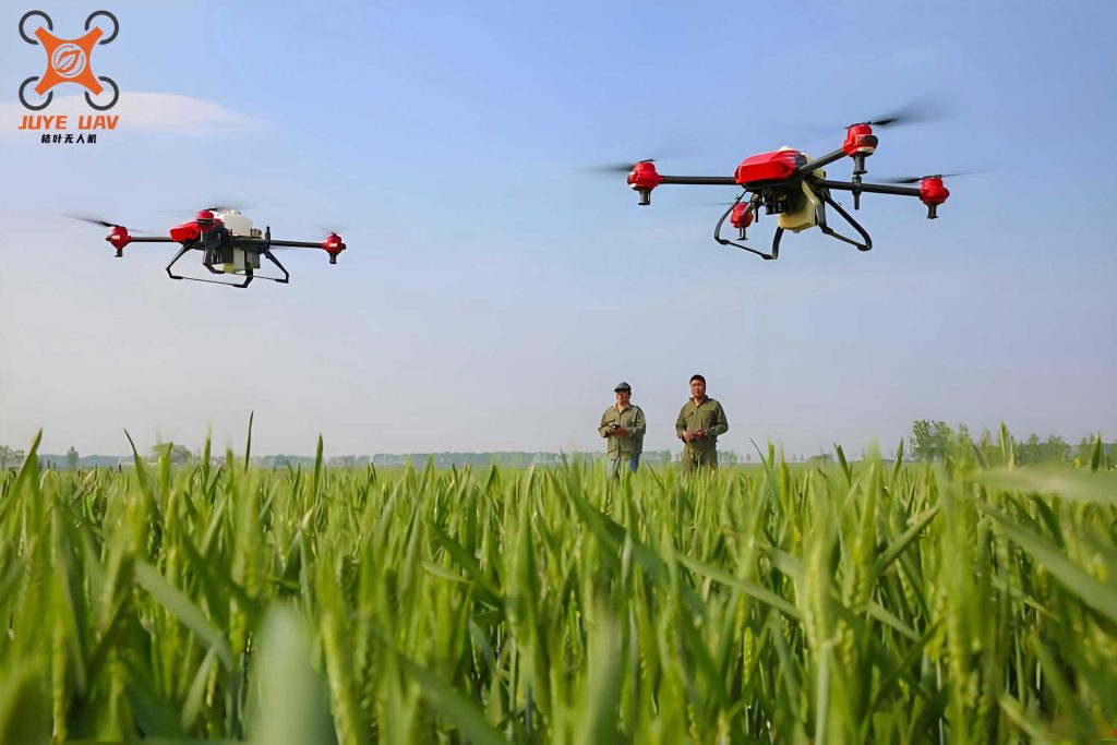
The evolution of modern agriculture increasingly relies on intelligent machinery to enhance efficiency, safety, and precision. Among these technologies, the agricultural drone has emerged as a transformative tool for tasks such as crop spraying, monitoring, and mapping. Particularly in challenging terrains like hills, mountains, and paddy fields, where traditional ground-based machinery faces significant access difficulties, the agricultural drone provides an unparalleled aerial platform for targeted operations. The core enabler for the autonomous and precise execution of these tasks is robust navigation and positioning technology. The performance of an agricultural drone is fundamentally constrained by the accuracy and reliability of its onboard localization and attitude estimation systems.
Conventional navigation solutions for agricultural drones often integrate Global Navigation Satellite Systems (GNSS) with Inertial Measurement Units (IMUs). However, GNSS signals can be weak or unavailable in environments with dense foliage or near geographical obstructions, leading to degraded or lost positioning. Furthermore, the inherent drift of low-cost IMUs, commonly used on agricultural drones for cost-effectiveness, accumulates rapidly, causing significant attitude and position errors over time. Therefore, developing advanced estimation algorithms that can fuse data from multiple sensors (like visual cameras, LiDAR, or radar) within a Simultaneous Localization and Mapping (SLAM) framework is critical for achieving the high-precision, stable navigation required for centimeter-accurate spraying and consistent flight path tracking.
The core mathematical challenge lies in the nonlinear nature of both the motion models (describing how the agricultural drone moves) and the observation models (describing how sensors perceive the environment). Traditional filtering approaches like the Extended Kalman Filter (EKF) linearize these models, introducing truncation errors that can lead to suboptimal performance or even filter divergence. More sophisticated nonlinear filters, such as the Unscented Kalman Filter (UKF) and the Central Difference Kalman Filter (CDKF), were developed to better handle these nonlinearities by propagating a set of carefully chosen sample points (sigma points) through the original nonlinear functions.
While UKF and CDKF offer improved accuracy over EKF, they belong to a class known as Sigma-Point Kalman Filters (SPKF) and can still face numerical instability issues, particularly when dealing with the high-dimensional state vectors common in SLAM problems for agricultural drones. The state vector in SLAM not only includes the drone’s pose (position and orientation) but also the estimated positions of numerous environmental landmarks. This leads to large covariance matrices whose properties (positive definiteness, symmetry) must be preserved throughout recursive calculations to ensure filter stability.
This is where the Square-Root Cubature Kalman Filter (SRCKF) presents a significant advantage. The SRCKF algorithm is built on a rigorous numerical integration rule—the third-degree spherical-radial cubature rule—to compute multivariate moment integrals encountered in Bayesian filtering. More importantly, it propagates and updates the square-root factors of the state error covariance matrix, rather than the full covariance matrix itself. This approach inherently guarantees the positive semi-definiteness of the covariance matrix, dramatically improves numerical stability, and reduces computational cost for high-dimensional states. For an agricultural drone operating in complex, variable conditions, these properties translate directly into more reliable, accurate, and consistent navigation estimates.
This article presents a comprehensive analysis and application of the SRCKF algorithm for the precise localization and attitude estimation of an agricultural drone operating in a simulated near-ground environment. We formulate the navigation problem within a SLAM framework, detail the mathematical derivation of the SRCKF, and compare its performance against other square-root sigma-point filters, namely the Square-Root UKF (SRUKF) and the Square-Root CDKF (SRCDKF). Extensive Monte Carlo simulation results demonstrate the superior performance of the SRCKF-based SLAM algorithm in terms of estimation accuracy, convergence speed, and robustness, ultimately validating its potential for enabling next-generation precision agriculture from the air.
Theoretical Foundations: SLAM Model and SRCKF Algorithm
SLAM Problem Formulation
For an agricultural drone navigating an unknown or partially known environment, the SLAM problem involves concurrently estimating the drone’s evolving pose and a map of its surroundings. The state vector at time \(k\) is typically composed of the vehicle state \( \mathbf{x}_v \) and the map state \( \mathbf{x}_m \), containing \(N\) landmark positions:
$$
\mathbf{x}_k = [\mathbf{x}_{v,k}^T, \mathbf{x}_{m,1}^T, \mathbf{x}_{m,2}^T, …, \mathbf{x}_{m,N}^T]^T
$$
The associated error covariance matrix encapsulates the uncertainty in the state estimate and the correlations between the drone pose and each landmark:
$$
\mathbf{P}_k = \begin{bmatrix}
\mathbf{P}_{vv,k} & \mathbf{P}_{vm,k} \\
\mathbf{P}_{vm,k}^T & \mathbf{P}_{mm,k}
\end{bmatrix}
$$
where \( \mathbf{P}_{vv} \) is the vehicle pose covariance, \( \mathbf{P}_{mm} \) is the landmark map covariance, and \( \mathbf{P}_{vm} \) is the cross-covariance between them. The system is described by a nonlinear discrete-time state transition model and an observation model:
$$
\begin{aligned}
\mathbf{x}_k &= f(\mathbf{x}_{k-1}, \mathbf{u}_k) + \mathbf{w}_{k-1} \\
\mathbf{z}_k &= h(\mathbf{x}_k) + \mathbf{v}_k
\end{aligned}
$$
Here, \( f(\cdot) \) is the nonlinear process function driven by control input \( \mathbf{u}_k \), \( h(\cdot) \) is the nonlinear measurement function, \( \mathbf{w}_k \sim \mathcal{N}(0, \mathbf{Q}_k) \) is the process noise, and \( \mathbf{v}_k \sim \mathcal{N}(0, \mathbf{R}_k) \) is the measurement noise.
Square-Root Cubature Kalman Filter (SRCKF) Derivation
The SRCKF provides an efficient and stable solution to the recursive Bayesian estimation problem for this nonlinear system. Its core innovation is the use of cubature points derived from the spherical-radial rule to approximate Gaussian-weighted integrals.
1. Cubature Rule and Point Calculation:
The filter approximates the standard Gaussian integral using \(2n\) equally weighted cubature points, where \(n\) is the state dimension. The basic points and weights are:
$$
\boldsymbol{\xi}_i = \sqrt{n} \, \mathbf{e}_i, \quad w_i = \frac{1}{2n}, \quad i = 1, 2, …, 2n
$$
where \( \{\mathbf{e}_i\} \) is the set of \(n\)-dimensional unit vectors and their negatives. For example, for \(n=3\), the points are \([\sqrt{3}, 0, 0]^T\), \([0, \sqrt{3}, 0]^T\), \([0, 0, \sqrt{3}]^T\), and their negatives.
2. Algorithm Steps:
Assume at time \(k-1\), we have the posterior state estimate \( \hat{\mathbf{x}}_{k-1|k-1} \) and the square-root factor of its error covariance \( \mathbf{S}_{k-1|k-1} \), such that \( \mathbf{P}_{k-1|k-1} = \mathbf{S}_{k-1|k-1} \mathbf{S}_{k-1|k-1}^T \).
a) Time Update (Prediction):
i. Calculate the cubature points for the previous state:
$$
\mathbf{X}_{i, k-1|k-1} = \mathbf{S}_{k-1|k-1} \boldsymbol{\xi}_i + \hat{\mathbf{x}}_{k-1|k-1}, \quad i=1,2,…,2n
$$
ii. Propagate the points through the process model:
$$
\mathbf{X}^*_{i, k|k-1} = f(\mathbf{X}_{i, k-1|k-1}, \mathbf{u}_k)
$$
iii. Compute the predicted state mean and the square-root factor of the predicted error covariance:
$$
\begin{aligned}
\hat{\mathbf{x}}_{k|k-1} &= \frac{1}{2n} \sum_{i=1}^{2n} \mathbf{X}^*_{i, k|k-1} \\
\mathbf{S}_{k|k-1} &= \text{Tria}\left( [\boldsymbol{\chi}^*_{k|k-1}, \mathbf{S}_{Q, k-1}] \right)
\end{aligned}
$$
where \( \boldsymbol{\chi}^*_{k|k-1} = \frac{1}{\sqrt{2n}} [\mathbf{X}^*_{1, k|k-1} – \hat{\mathbf{x}}_{k|k-1}, \, \mathbf{X}^*_{2, k|k-1} – \hat{\mathbf{x}}_{k|k-1}, \, …, \, \mathbf{X}^*_{2n, k|k-1} – \hat{\mathbf{x}}_{k|k-1}] \), \( \mathbf{Q}_{k-1} = \mathbf{S}_{Q, k-1} \mathbf{S}_{Q, k-1}^T \), and \(\text{Tria}(\cdot)\) denotes a triangularization operation (e.g., QR decomposition) that returns a square-root matrix.
b) Measurement Update (Correction):
i. Recalculate cubature points based on the predicted state:
$$
\mathbf{X}_{i, k|k-1} = \mathbf{S}_{k|k-1} \boldsymbol{\xi}_i + \hat{\mathbf{x}}_{k|k-1}
$$
ii. Propagate these points through the measurement model:
$$
\mathbf{Z}_{i, k|k-1} = h(\mathbf{X}_{i, k|k-1})
$$
iii. Compute the predicted measurement mean and the square-root of its innovation covariance:
$$
\begin{aligned}
\hat{\mathbf{z}}_{k|k-1} &= \frac{1}{2n} \sum_{i=1}^{2n} \mathbf{Z}_{i, k|k-1} \\
\mathbf{S}_{zz, k|k-1} &= \text{Tria}\left( [\boldsymbol{\mathcal{Z}}_{k|k-1}, \mathbf{S}_{R, k}] \right)
\end{aligned}
$$
where \( \boldsymbol{\mathcal{Z}}_{k|k-1} = \frac{1}{\sqrt{2n}} [\mathbf{Z}_{1, k|k-1} – \hat{\mathbf{z}}_{k|k-1}, \, …, \, \mathbf{Z}_{2n, k|k-1} – \hat{\mathbf{z}}_{k|k-1}] \) and \( \mathbf{R}_{k} = \mathbf{S}_{R, k} \mathbf{S}_{R, k}^T \).
iv. Compute the cross-covariance matrix and the Kalman gain:
$$
\begin{aligned}
\mathbf{P}_{xz, k|k-1} &= \boldsymbol{\chi}_{k|k-1} \boldsymbol{\mathcal{Z}}_{k|k-1}^T \\
\mathbf{K}_k &= (\mathbf{P}_{xz, k|k-1} / \mathbf{S}_{zz, k|k-1}^T) / \mathbf{S}_{zz, k|k-1}
\end{aligned}
$$
where \( \boldsymbol{\chi}_{k|k-1} = \frac{1}{\sqrt{2n}} [\mathbf{X}_{1, k|k-1} – \hat{\mathbf{x}}_{k|k-1}, \, …, \, \mathbf{X}_{2n, k|k-1} – \hat{\mathbf{x}}_{k|k-1}] \), and \(/\) denotes matrix right division (solving linear systems).
v. Update the state estimate and the square-root factor of its error covariance:
$$
\begin{aligned}
\hat{\mathbf{x}}_{k|k} &= \hat{\mathbf{x}}_{k|k-1} + \mathbf{K}_k (\mathbf{z}_k – \hat{\mathbf{z}}_{k|k-1}) \\
\mathbf{S}_{k|k} &= \text{Tria}\left( [\boldsymbol{\chi}_{k|k-1} – \mathbf{K}_k \boldsymbol{\mathcal{Z}}_{k|k-1}, \quad \mathbf{K}_k \mathbf{S}_{R, k}] \right)
\end{aligned}
$$
This square-root formulation is numerically stable and efficient, making it particularly suitable for the sustained, precise navigation demands of an agricultural drone.
Comparative Study of Nonlinear Filters for Agricultural Drone Navigation
To contextualize the advantages of the SRCKF for agricultural drone applications, it is essential to compare it with other prominent nonlinear filters. The following table summarizes the key characteristics of the EKF, UKF, CDKF, and CKF/SRCKF families.
| Filter | Core Principle | Key Advantage | Key Limitation for Agricultural Drones | Numerical Stability |
|---|---|---|---|---|
| EKF | First-order Taylor series linearization of nonlinear models. | Simple conceptual framework, computationally light for low dimensions. | Large linearization errors lead to significant estimation inaccuracies and potential divergence, especially during aggressive maneuvers. | Poor. Relies on Jacobian calculations; covariance matrix may lose positive definiteness. |
| UKF | Uses a deterministic set of sigma points to capture the mean and covariance of a distribution. | No need to compute Jacobians; achieves at least second-order accuracy for Gaussian distributions. | Number of sigma points scales linearly (2n+1). For large SLAM states, this increases computational load. Tuning parameters (scaling factors) can affect performance. | Moderate. Direct propagation of the full covariance matrix can lead to loss of positive definiteness over time. |
| CDKF | Based on polynomial interpolation using Stirling’s formula; a type of divided difference filter. | Similar accuracy to UKF; often has slightly faster convergence. No design parameters needed. | Computational complexity similar to UKF. Also propagates the full covariance matrix. | Moderate. Shares the same numerical stability concerns as UKF. |
| CKF / SRCKF | Based on the third-degree spherical-radial cubature rule for numerical integration. | Derived from a strict numerical integration rule. SRCKF propagates the square-root factor, guaranteeing stability and reducing computational cost for high-dimensional states. | The basic CKF shares complexity with UKF/CDKF. The SRCKF implementation requires careful matrix triangularization. | Excellent (SRCKF). The square-root formulation inherently maintains positive semi-definiteness, crucial for reliable long-term operation of an agricultural drone. |
The SRCKF synthesizes the strengths of the cubature integration approach with the robustness of square-root filtering, making it the most suitable candidate for high-fidelity state estimation in agricultural drone navigation systems where reliability is paramount.
Experimental Setup and Simulation Environment
To rigorously evaluate the performance of the proposed SRCKF-SLAM algorithm for an agricultural drone, a comprehensive simulation environment was established. The scenario mimics a typical near-ground spraying mission over undulating terrain.
Agricultural Drone Dynamics Model: A standard 3D kinematic model was used for the agricultural drone. The state vector for the vehicle included position \((p_x, p_y, p_z)\) and orientation (roll \(\phi\), pitch \(\theta\), yaw \(\psi\)) in the world frame. The control inputs were velocity and angular rates.
Sensor Configuration: The simulated agricultural drone was equipped with a proprioceptive sensor (IMU for motion prediction) and an exteroceptive sensor (a ranging/vision sensor for landmark observation within a SLAM framework).
Noise Parameters: Realistic noise characteristics were modeled to reflect typical low-cost sensors used on commercial agricultural drones.
$$
\mathbf{Q} = \text{diag}\left( (0.25)^2, (0.03)^2, (0.2)^2 \right), \quad \mathbf{R} = \text{diag}\left( (0.1)^2, (0.01)^2, (0.1)^2 \right)
$$
Mission Profile: The agricultural drone was tasked to follow a predefined path at a constant velocity of \(v = 3 \, \text{m/s}\). The simulation time was set to 4000 seconds to evaluate long-term stability. To ensure statistical significance, 20 independent Monte Carlo runs were conducted for each filtering algorithm (SRCKF, SRCDKF, SRUKF).
Initial Conditions: The initial state error was set to zero for position. For the critical attitude estimation test, a significant initial misalignment was introduced, particularly a large yaw error of \(10^\circ\), along with smaller roll (\(0.4^\circ\)) and pitch (\(0.8^\circ\)) errors, to evaluate the filter’s convergence capability under non-ideal startup conditions for the agricultural drone.
Results and Discussion
Position Estimation Accuracy
The primary metric for evaluating the navigation system of an agricultural drone is the accuracy of its estimated position relative to its true path. The Root Mean Square Error (RMSE) over 20 Monte Carlo runs was computed for the X (lateral), Y (longitudinal/forward), and Z (altitude) axes.
X-axis Estimation: The forward direction (Y-axis) is often the primary path of travel. The results showed that all square-root filters performed adequately, but the SRCKF-SLAM algorithm consistently yielded the lowest mean error. More importantly, its error trajectory exhibited the smallest variance, indicating superior stability. The SRCDKF showed marginally faster initial convergence than the SRUKF, but both were overtaken by the lower and steadier error profile of the SRCKF, which maintained an error approximately 0.5 meters lower on average.
Y-axis Estimation: On the forward axis, the agricultural drone’s position error is most critical for following crop rows. The SRCKF algorithm again demonstrated a clear advantage, producing the smallest and most stable error profile. The SRUKF and SRCDKF algorithms showed higher mean errors and greater fluctuations over the long simulation period.
Z-axis (Altitude) Estimation: Maintaining a constant altitude is vital for uniform spray deposition. All three algorithms maintained good performance for the initial phase of the simulation. However, as the mission progressed beyond 4000 seconds, the error for both SRUKF and SRCDKF began to increase noticeably due to accumulated numerical inaccuracies. In contrast, the SRCKF-SLAM algorithm maintained a very stable and near-constant altitude error, highlighting its numerical robustness for sustained agricultural drone operations.
| Algorithm | X-axis RMSE | Y-axis RMSE | Z-axis RMSE | Overall Stability |
|---|---|---|---|---|
| SRUKF-SLAM | Moderate, High Variance | Moderate, High Variance | Degrades over time | Least Stable |
| SRCDKF-SLAM | Moderate, Slightly Lower Variance | Moderate, Slightly Lower Variance | Degrades over time | Moderately Stable |
| SRCKF-SLAM | Lowest, Lowest Variance | Lowest, Lowest Variance | Consistently Low | Most Stable |
Attitude Estimation and Convergence
While position is critical, the attitude (orientation) of the agricultural drone directly impacts spray swath control, stability, and the geometric correctness of the built map in SLAM. A key test is the filter’s ability to converge from a large initial attitude error, simulating a poor initial alignment or a temporary sensor outage.
Given an initial misalignment of \([0.4^\circ, 0.8^\circ, 10^\circ]\) for roll, pitch, and yaw respectively, the SRCKF algorithm demonstrated exceptional performance. The small roll and pitch errors were corrected to near zero within seconds. Most impressively, the large \(10^\circ\) yaw error—which would cause a significant deviation in the agricultural drone’s heading and spraying path—was steadily estimated and corrected. The SRCKF drove this major yaw error to converge near zero within approximately 50 seconds. This rapid and accurate convergence is essential for an agricultural drone to recover its correct heading and resume precise, row-aligned flight after any disruption, ensuring complete and non-overlapping coverage of the crop area.
Conclusion and Future Work
This study presented a detailed investigation into high-precision navigation for agricultural drones using the Square-Root Cubature Kalman Filter within a SLAM framework. Through rigorous mathematical formulation and extensive simulation, the SRCKF-SLAM algorithm was demonstrated to outperform comparable square-root sigma-point filters (SRUKF and SRCDKF) in terms of positional estimation accuracy, long-term numerical stability, and convergence rate from large initial attitude errors. The ability of the SRCKF to maintain a stable and accurate estimate of the agricultural drone’s state, particularly in the critical yaw axis, directly translates to more reliable autonomous path following and precise application of agricultural inputs.
The inherent properties of the SRCKF—propagating the square-root of the covariance matrix and using a numerically rigorous cubature rule—make it uniquely suited for the demanding real-world conditions faced by agricultural drones, including long mission times, computational constraints, and the need for unwavering reliability. Future work will focus on implementing and validating this algorithm on a physical agricultural drone platform, integrating multi-sensor data (e.g., multi-spectral cameras, millimeter-wave radar) for robust perception in all weather and lighting conditions, and further optimizing the computational efficiency for real-time operation on embedded systems. The continuous advancement of such intelligent estimation algorithms is pivotal for unlocking the full potential of autonomous systems in precision agriculture, leading to increased efficiency, reduced chemical usage, and improved crop management.