In the evolving landscape of unmanned aerial systems, the capability to operate in complex, low-altitude environments has become a critical demand. I focus on a novel fixed-wing Vertical Take-Off and Landing Unmanned Aerial Vehicle (VTOL UAV), which combines the efficiency of fixed-wing cruise with the versatility of vertical take-off and landing. This VTOL UAV is particularly suited for missions in urban canyons or confined spaces where conventional runway access is limited. The transition maneuver—the phase where the VTOL UAV shifts between hover and forward flight—poses significant control challenges due to nonlinear dynamics, control redundancy, and coupling between aerodynamic surfaces and thrust vectoring. In this paper, I investigate a nonlinear optimal control allocation strategy for the six-degree-of-freedom transition maneuver, aiming to enhance tracking performance and maneuverability. The core of my approach lies in integrating Incremental Nonlinear Dynamic Inversion (INDI) with a two-stage cascaded optimal control allocation method, which efficiently handles control redundancies while mitigating model uncertainties. Throughout this study, the term VTOL UAV will be emphasized to underscore the platform’s unique characteristics and the broader applicability of the proposed methods to similar systems.
The transition maneuver for a VTOL UAV involves complex interactions between aerodynamic forces, thrust vectoring, and direct force control. During this phase, the VTOL UAV operates at low speeds where aerodynamic control surfaces become less effective, necessitating the use of thrust vectoring and direct forces for attitude and trajectory control. This results in an over-actuated system with multiple control effectors, including aerodynamic rudders, engine thrusts, and vectoring nozzles. The primary challenge is to allocate these control inputs optimally to achieve desired trajectory tracking while respecting physical constraints. I propose a global controller based on INDI, which linearizes the control model in incremental form, reducing sensitivity to aerodynamic model uncertainties. Subsequently, I develop a two-stage optimal control allocation framework that decomposes the allocation problem into trajectory and attitude loops, transforming nonlinear coupling issues into linear optimization problems. This method avoids iterative computations, enabling real-time implementation on onboard processors. Furthermore, I introduce a dynamic weighting strategy for the objective function, allowing the VTOL UAV to adjust allocation priorities based on flight states and mission requirements. The effectiveness of this approach is validated through extensive simulations of high-maneuverability transition paths, demonstrating robust tracking performance and adaptability. This research contributes to advancing control methodologies for VTOL UAVs, paving the way for more autonomous and capable systems in dynamic environments.
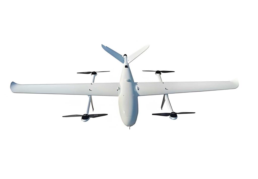
To contextualize this work, it is essential to understand the configuration of the VTOL UAV under study. The VTOL UAV features a tandem-wing lifting-body design, which provides increased lift within a limited wingspan, ideal for low-altitude operations. The propulsion system consists of one lift fan and two thrust-vectoring engines, enabling vertical take-off, transition, and cruise capabilities. The lift fan includes a control surface that can deflect laterally, providing side forces and yaw moments, while the engine vector nozzles can pivot to generate thrust components in multiple axes and control moments. This configuration introduces redundancy, as both aerodynamic and thrust-vectoring forces can influence the same degrees of freedom. Key parameters of the VTOL UAV are summarized in Table 1, which outlines its basic specifications critical for control design.
| Parameter | Value |
|---|---|
| Take-off speed (runway) | 15 m/s |
| Cruise speed | 20 m/s |
| Fuselage length | 1 m |
| Rear wingspan | 1.57 m |
| Mass | 5 kg |
| Maximum engine thrust | 26 N |
| Maximum lift fan thrust | 38 N |
| Range | 6 km |
The aerodynamic model for this VTOL UAV incorporates uncertainties due to factors like ground effect during vertical take-off, turbulent flow at high angles of attack, engine suction effects, and thrust losses from vector nozzle deflections. I represent aerodynamic forces and moments using polynomial approximations derived from computational fluid dynamics simulations and parameter identification, facilitating control allocation computations. For instance, the aerodynamic coefficients can be expressed as:
$$C_d = C_{d0} + C_{d\alpha} \alpha,$$
$$C_c = C_{c0} + C_{c\beta} \beta,$$
$$C_l = C_{l0} + C_{l\alpha} \alpha,$$
where \(C_d\), \(C_c\), and \(C_l\) are the drag, side-force, and lift coefficients, respectively; \(C_{d0}\), \(C_{c0}\), and \(C_{l0}\) are base coefficients subject to estimation errors; and \(C_{d\alpha}\), \(C_{c\beta}\), and \(C_{l\alpha}\) are dynamic derivatives assumed to be accurately known. Similar polynomial forms are used for moments. These representations are integral to the INDI controller, which mitigates uncertainties by focusing on incremental changes.
My control strategy is built upon the Incremental Nonlinear Dynamic Inversion (INDI) method, which offers robustness against model inaccuracies. I structure the control system into four loops based on time-scale separation: flight path kinematics, flight path dynamics, attitude kinematics, and attitude dynamics. The INDI approach is applied to the flight path and attitude dynamics loops, where uncertainties are most prevalent, while the kinematics loops use standard NDI. This hierarchical design ensures stability and performance across the VTOL UAV’s flight envelope.
For the flight path dynamics loop, the state vector is defined as \(\mathbf{x}_1 = [v, \chi, \gamma]^T\), where \(v\) is airspeed, \(\chi\) is flight path azimuth, and \(\gamma\) is flight path angle. The control vector is \(\mathbf{x}_2 = [\alpha, \beta, \mu, T_x, T_y, T_z]^T\), comprising angle of attack \(\alpha\), sideslip angle \(\beta\), flight path bank angle \(\mu\), and thrust components in the body frame \(T_x\), \(T_y\), and \(T_z\). The dynamics are governed by:
$$\dot{\mathbf{x}}_1 = \mathbf{f}_1(\mathbf{x}_1) + \mathbf{g}_1(\mathbf{x}_1, \mathbf{x}_2),$$
where \(\mathbf{f}_1\) represents gravity effects, and \(\mathbf{g}_1\) encompasses aerodynamic and thrust forces. Using INDI, I linearize this equation in incremental form. Denoting \(\mathbf{x}_{1n} = \mathbf{x}_1 + \Delta \mathbf{x}_1\) and \(\mathbf{x}_{2n} = \mathbf{x}_2 + \Delta \mathbf{x}_2\), and applying a first-order Taylor expansion while ignoring higher-order terms, I obtain:
$$\dot{\mathbf{x}}_{1n} – \dot{\mathbf{x}}_1 = \mathbf{g}_1(\mathbf{x}_1, \mathbf{x}_2 + \Delta \mathbf{x}_2) – \mathbf{g}_1(\mathbf{x}_1, \mathbf{x}_2).$$
This simplifies to a linear equation in increments:
$$\dot{\mathbf{x}}_1^d – \dot{\mathbf{x}}_{1f} = \begin{bmatrix} \mathbf{g}_{1a} & \mathbf{0} \\ \mathbf{0} & \mathbf{g}_{1t} \end{bmatrix} \begin{bmatrix} \Delta \mathbf{x}_{2a} \\ \Delta \mathbf{x}_{2t} \end{bmatrix},$$
where \(\dot{\mathbf{x}}_1^d\) is the desired derivative from a linear controller, \(\dot{\mathbf{x}}_{1f}\) is the filtered derivative of measured states, \(\mathbf{g}_{1a}\) and \(\mathbf{g}_{1t}\) are control effectiveness matrices for aerodynamic angles and thrust components, and \(\Delta \mathbf{x}_{2a} = [\Delta \alpha, \Delta \beta, \Delta \mu]^T\), \(\Delta \mathbf{x}_{2t} = [\Delta T_x, \Delta T_y, \Delta T_z]^T\). The use of filtered signals ensures temporal consistency and reduces noise sensitivity. The incremental control allocation problem then becomes:
$$\min_{\Delta \mathbf{x}_2} \|\mathbf{W}_1 (\Delta \mathbf{x}_2 + \mathbf{x}_{2f})\|^2 + \|\mathbf{W}_2 \Delta \mathbf{x}_2\|^2, \quad \text{subject to} \quad \begin{bmatrix} \mathbf{g}_{1a} & \mathbf{0} \\ \mathbf{0} & \mathbf{g}_{1t} \end{bmatrix} \Delta \mathbf{x}_2 = \boldsymbol{\nu},$$
with \(\boldsymbol{\nu} = \dot{\mathbf{x}}_1^d – \dot{\mathbf{x}}_{1f}\). Here, \(\mathbf{W}_1\) and \(\mathbf{W}_2\) are dynamic weighting matrices that prioritize control magnitudes and rates, respectively. This formulation decouples the nonlinear allocation into a linear constrained optimization, solvable via weighted pseudo-inverse methods without iteration. The solution is given by:
$$\Delta \mathbf{x}_2 = \mathbf{G} \boldsymbol{\nu} + (\mathbf{G} \mathbf{B} – \mathbf{I}) \mathbf{x}_{20},$$
where \(\mathbf{B} = \begin{bmatrix} \mathbf{g}_{1a} & \mathbf{0} \\ \mathbf{0} & \mathbf{g}_{1t} \end{bmatrix}\), \(\mathbf{G} = \mathbf{W}^{-1} (\mathbf{B} \mathbf{W}^{-1})^\dagger\), \(\mathbf{W} = \sqrt{\mathbf{W}_1^2 + \mathbf{W}_2^2}\), and \(\mathbf{x}_{20} = \mathbf{W}^{-2} (\mathbf{W}_1^2 \mathbf{x}_{2f})\). This approach significantly reduces computational load, making it suitable for real-time implementation on VTOL UAV platforms.
The attitude dynamics loop follows a similar INDI structure. The state vector is \(\mathbf{x}_3 = [p, q, r]^T\), representing body-axis angular rates, and the control vector is \(\mathbf{x}_4 = [l_c, m_c, n_c]^T\), the control moments. The dynamics are:
$$\dot{\mathbf{x}}_3 = \mathbf{f}_3(\mathbf{x}_3) + \mathbf{J}^{-1} \mathbf{x}_4,$$
with \(\mathbf{J}\) as the inertia matrix. Applying INDI yields:
$$\Delta \mathbf{x}_4 = \mathbf{J} (\dot{\mathbf{x}}_3^d – \dot{\mathbf{x}}_{3f}),$$
where \(\dot{\mathbf{x}}_{3f}\) is the filtered angular acceleration. The incremental moment \(\Delta \mathbf{x}_4\) is then allocated to aerodynamic and thrust-vectoring moments in the second stage of control allocation.
To manage the redundancy and coupling in control allocation for the VTOL UAV, I propose a two-stage cascaded optimal control allocation method. This method coordinates the trajectory and attitude loops, ensuring that control efforts are distributed efficiently among all effectors. The first stage handles allocation in the flight path dynamics loop, producing incremental thrust components \(\Delta \mathbf{x}_{2t}\) and aerodynamic angles \(\Delta \mathbf{x}_{2a}\). The second stage allocates these increments along with the incremental moments \(\Delta \mathbf{x}_4\) to the actual actuators: engine thrusts \(\mathbf{T}_e = [T_l, T_r, T_f]^T\), vector nozzle angles \(\boldsymbol{\delta}_{tvn} = [\delta_l, \delta_r, \delta_f]^T\), and aerodynamic rudder angles \(\boldsymbol{\delta}_{as} = [\delta_a, \delta_e, \delta_r]^T\).
In the first stage, I employ a dynamic weighted pseudo-inverse method with a self-adjusting weight selection strategy. The weights in \(\mathbf{W}_1\) and \(\mathbf{W}_2\) are determined using a hierarchical analytic process that considers flight conditions and mission requirements. For instance, at low speeds, thrust vectoring may be prioritized over aerodynamic control, whereas at higher speeds, the reverse may be true. I define weight structures with three layers: top-level sets (e.g., aerodynamic vs. thrust), sub-level sets (e.g., angles vs. rates), and element-level weights. The weights are normalized and adjusted online based on saturation counts to ensure smooth transitions. This dynamic weighting allows the VTOL UAV to adapt its control strategy seamlessly during transition maneuvers.
The second stage allocation combines the increments from both loops. The thrust and moment contributions from the propulsion system are modeled as:
$$\mathbf{x}_{2t} = \begin{bmatrix} T_l \cos \delta_l + T_r \cos \delta_r \\ T_f \sin \delta_f \\ T_l \sin \delta_l + T_r \sin \delta_r – T_f \cos \delta_f \end{bmatrix},$$
$$\mathbf{x}_{4t} = \begin{bmatrix} -T_l d_{yt} \sin \delta_l + T_r d_{yt} \sin \delta_r \\ (T_l \sin \delta_l + T_r \sin \delta_r) d_{xt} + T_f d_{xf} \cos \delta_f \\ (T_l \cos \delta_l – T_r \cos \delta_r) d_{yt} + T_f d_{xf} \sin \delta_f \end{bmatrix},$$
where \(d_{xt}\), \(d_{xf}\), and \(d_{yt}\) are distances from actuators to the center of mass. Linearizing these equations in incremental form, and ignoring higher-order terms, gives:
$$\begin{bmatrix} \Delta \mathbf{x}_{2t} \\ \Delta \mathbf{x}_{4t} \end{bmatrix} = \mathbf{G}_e \begin{bmatrix} \Delta \mathbf{T}_e \\ \Delta \boldsymbol{\delta}_{tvn} \end{bmatrix},$$
where \(\mathbf{G}_e\) is a \(6 \times 6\) matrix dependent on current actuator states. By inverting \(\mathbf{G}_e\), I compute the increments for thrusts and vector angles. Aerodynamic rudder increments are derived separately using a chained approach, where aerodynamic moments are prioritized: \(\Delta \boldsymbol{\delta}_{as} = \Delta \mathbf{x}_{4s} / (q S \mathbf{b}_1 \mathbf{C}_{as})\), with \(q\) as dynamic pressure, \(S\) reference area, \(\mathbf{b}_1\) a diagonal matrix of dimensions, and \(\mathbf{C}_{as}\) the control effectiveness matrix for rudders. This two-stage method transforms a nonlinear, coupled allocation into linear steps, avoiding iterative solvers and enhancing real-time feasibility for VTOL UAV applications.
To validate the proposed control allocation framework for the VTOL UAV, I conduct simulation studies of a high-maneuverability transition trajectory. The reference path is designed to showcase six-degree-of-freedom capabilities: acceleration along the north axis, periodic lateral motion along the east axis, and altitude variations. Specifically, the velocity components in the ground frame are:
$$v_x = t/5, \quad v_y = (t/12) \cos(2\pi t/30), \quad v_z = -2 \cos(2\pi t/120),$$
with time \(t\) in seconds. The VTOL UAV starts from hover and tracks this path, demonstrating transition from vertical to forward flight with aggressive maneuvers. I evaluate two weighting schemes to illustrate adaptability: Scheme 1 emphasizes direct force control for smoother attitude changes, suitable for manned VTOL UAV operations; Scheme 2 prioritizes aerodynamic control for larger attitude maneuvers, typical of small unmanned VTOL UAVs. The simulation parameters are listed in Table 2, including controller gains and filter settings.
| Parameter | Value |
|---|---|
| Control frequency | 100 Hz |
| Filter damping ratio \(\zeta\) | 0.7 |
| Filter natural frequency \(\omega_n\) | 50 rad/s |
| Flight path control gain \(\mathbf{K}_1\) | diag(2, 2, 2) |
| Attitude control gain \(\mathbf{K}_3\) | diag(5, 5, 5) |
| Weight adjustment threshold | 300 counts |
The simulation results, summarized in Table 3, show key performance metrics for both weighting schemes. Scheme 1 achieves better trajectory tracking with smaller attitude deviations, while Scheme 2 exhibits larger angles but reduced direct force usage. Both schemes successfully track the reference path, with root-mean-square errors in position below 0.5 m, confirming the effectiveness of the INDI-based control allocation for the VTOL UAV.
| Metric | Scheme 1 | Scheme 2 |
|---|---|---|
| Max angle of attack \(\alpha\) | 22.3° | 66.21° |
| Max pitch angle \(\theta\) | 13.36° | 58.68° |
| Lift fan usage | Continuous | Intermittent |
| Position RMSE | 0.21 m | 0.45 m |
| Control effort (norm) | Low | High |
Additionally, I analyze the robustness of the INDI controller by introducing external disturbances to simulate wind gusts. The disturbance force is modeled as \(\mathbf{F}_d = 6 R \sin(0.05\pi t)\), where \(R\) is a random number between 0 and 3 updated every 3 seconds. Compared to a standard NDI controller with sequential quadratic programming allocation, the INDI controller shows superior disturbance rejection, with position deviations reduced by over 50% in simulations. This highlights the advantage of INDI in handling uncertainties for VTOL UAV operations.
The control allocation process involves numerous equations. To summarize, the overall dynamics of the VTOL UAV can be represented in a compact form. The translational dynamics are:
$$\mathbf{M} \dot{\mathbf{v}} = \mathbf{F}_a + \mathbf{F}_t + \mathbf{F}_g,$$
where \(\mathbf{M}\) is the mass matrix, \(\mathbf{v}\) is the velocity vector, \(\mathbf{F}_a\) are aerodynamic forces, \(\mathbf{F}_t\) are thrust forces, and \(\mathbf{F}_g\) is gravity. The rotational dynamics are:
$$\mathbf{J} \dot{\boldsymbol{\omega}} = \mathbf{M}_a + \mathbf{M}_t – \boldsymbol{\omega} \times \mathbf{J} \boldsymbol{\omega},$$
with \(\boldsymbol{\omega}\) as angular velocity, \(\mathbf{M}_a\) aerodynamic moments, and \(\mathbf{M}_t\) thrust-vectoring moments. The INDI controller linearizes these equations around the current state, yielding incremental relationships. For example, the thrust force increments relate to actuator increments as:
$$\Delta \mathbf{F}_t = \frac{\partial \mathbf{F}_t}{\partial \mathbf{T}_e} \Delta \mathbf{T}_e + \frac{\partial \mathbf{F}_t}{\partial \boldsymbol{\delta}_{tvn}} \Delta \boldsymbol{\delta}_{tvn}.$$
These partial derivatives form the \(\mathbf{G}_e\) matrix, enabling efficient allocation. The optimization problem in the first stage can be generalized as:
$$\min_{\Delta \mathbf{u}} \| \mathbf{Q} (\Delta \mathbf{u} + \mathbf{u}_0) \|^2 \quad \text{s.t.} \quad \mathbf{A} \Delta \mathbf{u} = \mathbf{b},$$
where \(\mathbf{u}\) represents control variables, \(\mathbf{Q}\) is a weighting matrix, \(\mathbf{A}\) is the control effectiveness matrix, and \(\mathbf{b}\) is the desired increment. The solution is \(\Delta \mathbf{u} = \mathbf{A}^\dagger \mathbf{b} + (\mathbf{I} – \mathbf{A}^\dagger \mathbf{A}) \mathbf{u}_0\), with \(\dagger\) denoting the weighted pseudo-inverse. This framework is applicable to various VTOL UAV configurations beyond the studied platform.
In conclusion, I have developed and validated a comprehensive control allocation strategy for fixed-wing VTOL UAVs during transition maneuvers. The integration of INDI control with a two-stage optimal allocation addresses nonlinearities, redundancies, and uncertainties inherent in VTOL UAV dynamics. Key contributions include: (1) an INDI-based global controller that reduces sensitivity to aerodynamic model errors; (2) a cascaded allocation method that transforms nonlinear problems into linear optimizations, avoiding iterative computations; and (3) a dynamic weighting strategy that adapts to flight states and mission needs. Simulations demonstrate that the VTOL UAV can track aggressive six-degree-of-freedom paths with high accuracy, leveraging both direct force and aerodynamic control. The methods are computationally efficient, making them suitable for real-time implementation on embedded systems. Future work will focus on experimental validation with a physical VTOL UAV prototype and extension to multi-agent cooperative scenarios. This research underscores the potential of advanced control techniques to enhance the autonomy and versatility of VTOL UAVs in complex environments.
To further illustrate the mathematical foundations, consider the error dynamics of the VTOL UAV under INDI control. Defining the tracking error \(\mathbf{e} = \mathbf{x} – \mathbf{x}^d\), the closed-loop system can be expressed as:
$$\dot{\mathbf{e}} + \mathbf{K} \mathbf{e} = \mathbf{d},$$
where \(\mathbf{K}\) is the controller gain matrix, and \(\mathbf{d}\) represents bounded disturbances due to model uncertainties. Using Lyapunov analysis, one can show that \(\|\mathbf{e}\|\) converges to a small region around zero, ensuring stability for the VTOL UAV. The control allocation weights play a crucial role in minimizing \(\mathbf{d}\) by optimizing control efforts. For instance, the weight update law based on saturation counts can be formulated as:
$$w_{ijk}(t+1) = w_{ijk}(t) + \eta \cdot \text{sat}_{ijk}(t),$$
where \(\eta\) is a small positive constant, and \(\text{sat}_{ijk}(t)\) indicates saturation events for control variable \(ijk\). This adaptive mechanism ensures that the VTOL UAV continuously refines its allocation strategy during flight.
In summary, this study provides a robust framework for controlling VTOL UAVs in transition maneuvers, with wide applications in surveillance, delivery, and emergency response. The emphasis on VTOL UAV capabilities highlights the importance of tailored control solutions for next-generation aerial systems. The proposed methods are scalable and adaptable, promising to advance the state-of-the-art in unmanned aviation.