The evolution of unmanned aerial systems demands platforms with increasingly versatile flight envelopes. Among these, the Vertical Take-Off and Landing (VTOL) drone that integrates ducted lift fans with a fixed-wing airframe represents a significant technological advancement. This configuration marries the helicopter’s invaluable capabilities of hovering, vertical ascent/descent, and low-speed maneuverability with the fixed-wing aircraft’s superior efficiency and endurance for high-speed cruise. The operational flexibility offered by such a VTOL drone opens vast application potentials in both civilian and military domains, from infrastructure inspection and precision agriculture to reconnaissance and logistics. Consequently, a deep understanding of its flight dynamics, particularly during the critical transition phase between hovering and forward flight, is paramount for safe and reliable design and operation.
The flight regime of a duct VTOL drone can be distinctly partitioned into three phases: the hover/low-speed vertical flight phase, the high-speed forward flight phase, and the intricate transition phase that bridges the two. The transition phase is arguably the most complex and demanding. During this period, the vehicle’s aerodynamic configuration undergoes a continuous transformation. The lift generation shifts from being predominantly thrust-borne (from the lift fan and tilted thrust ducts) to being primarily wing-borne. Simultaneously, control authority must be seamlessly transferred from differential thrust or vanes to conventional aerodynamic control surfaces. This dynamic reconfiguration necessitates precise management of power distribution, attitude, and airspeed to ensure that net lift always compensates for weight and that the vehicle remains controllable. Defining a safe “transition corridor”—a set of permissible airspeed and attitude combinations—and ensuring inherent or augmented stability within this corridor are therefore central challenges in the development of a robust VTOL drone.
This article presents a detailed investigation into the longitudinal flight dynamics and stability of a composite VTOL drone featuring a forward-mounted coaxial ducted lift fan and rear-mounted, tiltable thrust ducts. The core of this study lies in developing high-fidelity yet computationally tractable aerodynamic models for the unique propulsive components and integrating them into a full six-degree-of-freedom (6-DOF) nonlinear flight dynamics model. The longitudinal stability across hover and transition states is then rigorously analyzed using linearization techniques and eigenvalue analysis. A case study on a specific VTOL drone configuration validates the modeling approach, with stability predictions corroborated by experimental hover test data.
1. System Description and Reference Frames
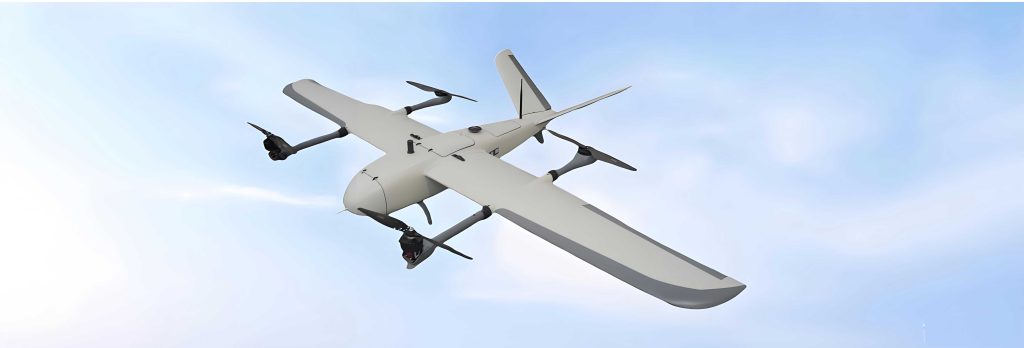
The subject of this study is a tail-sitter type VTOL drone. Its primary propulsion system consists of two key elements: a large-diameter, coaxial counter-rotating ducted fan (the lift fan) positioned forward of the vehicle’s center of gravity (CG), and two smaller-diameter, tiltable ducted fans (the thrust ducts) mounted near the trailing edge of the fixed wing. The lift fan provides the bulk of the vertical thrust. The thrust ducts serve a dual purpose: in hover, they are tilted to contribute to vertical lift and provide pitch/yaw control moments; during transition and forward flight, they are progressively tilted forward to generate axial thrust for propulsion.
To analyze the vehicle’s motion, two right-handed coordinate systems are primarily employed:
1. Earth-Fixed Inertial Frame (OEXEYEZE): Origin at an arbitrary point on ground. XE points North, YE points East, and ZE points down towards the center of the Earth.
2. Body-Fixed Frame (ObXbYbZb): Origin at the vehicle’s CG. Xb axis points forward along the fuselage reference line, Yb axis points to the right (starboard), and Zb axis points downward to complete the right-handed system, lying in the aircraft’s plane of symmetry. This is the primary frame for expressing forces, moments, and translational/rotational velocities.
The state variables for longitudinal motion are defined within the body frame: translational velocities u (forward) and w (downward), angular rate q (pitch rate), and the Euler pitch angle $\theta$. The angle of attack $\alpha$ is derived as $\alpha = \arctan(w/u)$.
2. Aerodynamic Modeling of Propulsive Components
Accurate modeling of the ducted fan systems is critical, as their performance dictates the vehicle’s capabilities in hover and low-speed flight. The modeling approach combines first-principles Blade Element Momentum Theory (BEMT) with empirical corrections derived from Computational Fluid Dynamics (CFD) and static thrust test data. This hybrid method ensures physical fidelity while maintaining computational efficiency suitable for dynamics analysis.
2.1 Coaxial Ducted Lift Fan Model
The coaxial counter-rotating lift fan offers significant advantages over a single rotor: it inherently cancels reactive torque, improves hover efficiency by recovering swirl energy from the upper rotor, and allows for a more compact design for a given thrust requirement. However, the presence of the duct and the interaction between the two rotors complicate the flow field. The duct lip generates additional suction-based thrust, and the lower rotor operates partially within the contracted wake of the upper rotor.
The proposed model adapts classical BEMT for coaxial rotors. The key assumptions are: the upper rotor’s wake affects the inflow of the lower rotor, but not vice-versa; the wake contracts to a known area ratio at the plane of the lower rotor; and the duct’s primary effect on the rotors is to modify the induced inflow, particularly for the upper rotor. Instead of performing a full radial integration for every calculation, a characteristic section method is employed. The aerodynamic properties at a representative radial station (e.g., $r/R = 0.7$) are used to characterize the performance of the entire rotor disk, significantly simplifying the model for stability derivative calculation. Correction factors ($\eta$) are introduced based on experimental data to account for duct lip effects and other discrepancies from ideal theory.
The inflow velocity at the characteristic section of the upper rotor is calculated as:
$$\lambda_u^{fan} = \sqrt{ \left( \frac{\sigma_u C_{l\alpha}}{16 F} – \frac{\lambda_{\infty}}{2} \right)^2 + \frac{\sigma_u C_{l\alpha}}{8 F} \theta_u r } – \left( \frac{\sigma_u C_{l\alpha}}{16 F} – \frac{\lambda_{\infty}}{2} \right) \cdot \eta(V_{\infty})$$
where $\lambda = v/(\Omega R)$ is the non-dimensional induced inflow, $\lambda_{\infty}=V_{\infty}/(\Omega R)$ is the non-dimensional freestream velocity, $\sigma$ is solidity, $C_{l\alpha}$ is the airfoil lift curve slope, $\theta$ is the blade pitch angle at the characteristic section, $r$ is the non-dimensional radius, $F$ is the Prandtl tip loss factor, and $\eta$ is the empirical duct correction factor, which is a function of the local axial flow $V_{\infty}$.
The thrust coefficient for the upper rotor characteristic section is then:
$$C_{T_u} = \frac{1}{2} \sigma_u C_{l\alpha} (\theta_u r^2 – \lambda_u^{fan} r)$$
For the lower rotor, the inflow is calculated considering it operates in the wake of the upper rotor ($\lambda_u^{fan}$). The wake contraction is modeled, and the inflow equation is solved similarly. The thrust coefficient $C_{T_l}$ is computed analogously. The total thrust $T_{fan}$ from the lift fan is:
$$T_{fan} = \rho A_{fan} (\Omega R)_{fan}^2 (C_{T_u} + C_{T_l})$$
where $\rho$ is air density and $A_{fan}$ is the fan disk area.
2.2 Tiltable Thrust Duct Model
The thrust ducts are modeled as single-rotor ducted fans. They typically have a higher rotational speed and lower solidity than the lift fan. The stator (fixed downstream blades) is not modeled as a separate lifting element but its effect is lumped into an overall efficiency and swirl recovery correction. The modeling philosophy is similar: a characteristic section BEMT approach with empirical duct corrections.
The inflow for the thrust duct rotor is given by:
$$\lambda_u^{duct} = \sqrt{ \left( \frac{\sigma_u C_{l\alpha}}{16} – \frac{\lambda_{\infty, duct}}{2} \right)^2 + \frac{\sigma_u C_{l\alpha}}{8} \theta_u r } – \left( \frac{\sigma_u C_{l\alpha}}{16} – \frac{\lambda_{\infty, duct}}{2} \right) \cdot \eta_{duct}$$
Note the absence of the tip loss factor $F$ due to the ducted configuration minimizing tip losses. The freestream velocity for the duct, $V_{\infty,duct}$, is a function of the vehicle’s body velocities ($u$, $w$), its pitch rate $q$, the duct’s tilt angle $\delta_d$, and its distance from the CG ($L_{duct}$):
$$V_{\infty,duct} = – (w + q L_{duct}) \sin\delta_d + u \cos\delta_d$$
The thrust is then:
$$T_{duct} = \rho A_{duct} (\Omega R)_{duct}^2 C_{T_u}$$
The following table summarizes the key parameters for the aerodynamic models of the propulsive components for the case study vehicle.
| Component | Parameter | Symbol | Value / Description |
|---|---|---|---|
| Lift Fan | Diameter | D_fan | 0.46 m |
| Characteristic Section | r/R | 0.7 | |
| Blade Solidity (Upper/Lower) | σ_u, σ_l | 0.15, 0.15 | |
| Duct Correction Factor | η(V∞) | Empirical function from test data | |
| Reference Area | A_fan | π*(0.23)^2 m² | |
| Thrust Duct | Diameter | D_duct | 0.07 m |
| Characteristic Section | r/R | 0.7 | |
| Blade Solidity | σ | 0.25 | |
| Duct Correction Factor | η_duct | Empirical constant | |
| Tilt Angle Range | δ_d | 0° (forward) to 90° (upward) |
3. Integrated Flight Dynamics Model
The full nonlinear equations of motion for a rigid-body VTOL drone are established in the body frame. The model must account for the tilt of the thrust ducts, which not only changes the direction of their force vector but also slightly alters the vehicle’s moment of inertia about the pitch axis as their mass rotates relative to the CG. The longitudinal equations are extracted for stability analysis.
The forces and moments acting on the vehicle are the sum of contributions from:
- Gravity (resolved in the body axis).
- Lift Fan (thrust along $+Z_b$, moment due to longitudinal offset).
- Thrust Ducts (thrust depends on tilt angle $\delta_d$, moments due to offset).
- Wing/Body Aerodynamics (lift, drag, and pitching moment, functions of $\alpha$ and airspeed $V=\sqrt{u^2+w^2}$).
The nonlinear longitudinal force and moment equations are:
$$m(\dot{u} + q w) = -mg\sin\theta + F_{x,fan} + F_{x,duct}(\delta_d) + F_{x,aero}(\alpha, V)$$
$$m(\dot{w} – q u) = mg\cos\theta + F_{z,fan} + F_{z,duct}(\delta_d) + F_{z,aero}(\alpha, V)$$
$$I_{yy}\dot{q} = M_{fan} + M_{duct}(\delta_d) + M_{aero}(\alpha, V, q)$$
where $m$ is mass, $g$ is gravity, and $I_{yy}$ is the time-varying pitch moment of inertia $I_{yy}(\delta_d)$. The kinematic relation for pitch angle is $\dot{\theta} = q$.
For stability analysis, these equations are linearized about a reference equilibrium (trim) flight condition. The state vector for longitudinal motion is $\mathbf{x} = [\Delta u, \Delta w, \Delta q, \Delta \theta]^T$, where $\Delta$ denotes a small perturbation from the trim value. The linearized system takes the standard state-space form:
$$\mathbf{A} \dot{\mathbf{x}} = \mathbf{B} \mathbf{x} \quad \Rightarrow \quad \dot{\mathbf{x}} = \mathbf{A}_s \mathbf{x}, \quad \mathbf{A}_s = \mathbf{A}^{-1}\mathbf{B}$$
The matrices $\mathbf{A}$ and $\mathbf{B}$ are:
$$\mathbf{A} = \begin{bmatrix}
m & 0 & 0 & 0\\
0 & m & 0 & 0\\
0 & 0 & I_{yy} & 0\\
0 & 0 & 0 & 1
\end{bmatrix}$$
$$\mathbf{B} = \begin{bmatrix}
X_u & X_w & X_q – m w_0 & -mg\cos\theta_0\\
Z_u & Z_w & Z_q + m u_0 & -mg\sin\theta_0\\
M_u & M_w & M_q & 0\\
0 & 0 & 1 & 0
\end{bmatrix}$$
where the subscript notation denotes stability derivatives (e.g., $X_u = \frac{\partial F_x}{\partial u}$). These derivatives are calculated analytically or via numerical perturbation from the combined aerodynamic model comprising the fan, ducts, and wing. The eigenvalues of the system matrix $\mathbf{A}_s$ determine the longitudinal dynamic modes and their stability.
4. Case Study: Trim and Stability Analysis
The developed modeling framework is applied to a specific VTOL drone with a mass of 9.2 kg. The key steps involve solving for trim conditions in hover and transition, and then performing an eigenvalue analysis.
4.1 Trim Analysis
Hover Trim: In pure hover, the wing aerodynamics are negligible. The trim equations solve for lift fan thrust ($T_{fan}$), thrust duct thrust ($T_{duct}$), and duct tilt angle ($\delta_d$) for a given vehicle pitch attitude ($\theta$).
$$T_{duct}\cos\delta_d – mg\sin\theta = 0$$
$$T_{fan} + T_{duct}\sin\delta_d – mg\cos\theta = 0$$
$$T_{fan} l_{fan} – T_{duct} l_{duct} \sin\delta_d = 0$$
where $l$ denotes the longitudinal moment arm from the CG. The solution provides the control settings required to maintain a stationary hover at a non-zero pitch angle.
Transition Trim: During transition, wing aerodynamics become significant. The trim equations now balance forces and moments including wing lift ($L_w$), drag ($D_w$), and pitching moment ($M_w$).
$$T_{duct}\cos\delta_d + L_w\sin\theta – D_w\cos\theta – mg\sin\theta = 0$$
$$T_{fan} + T_{duct}\sin\delta_d + L_w\cos\theta + D_w\sin\theta – mg\cos\theta = 0$$
$$M_w + T_{fan} l_{fan} – T_{duct} l_{duct} \sin\delta_d = 0$$
Solving these for a range of airspeeds yields the required variation in thrusts and duct angle to maintain steady flight at a constant pitch attitude.
Trim results for the case study vehicle show that as forward speed increases from hover, the required thrust from the lift fan decreases monotonically as the wing takes over lift generation, while the thrust ducts progressively tilt forward to provide propulsive thrust.
4.2 Longitudinal Stability Analysis
The stability derivatives are populated using the aerodynamic models. The accuracy of the lift fan model is first verified against static test data, showing a deviation of less than 5% across the operational range, which is deemed acceptable for dynamics analysis.
Hover Stability: The eigenvalues of the linearized system are computed for hover trim conditions at different pitch attitudes ($\theta$). The results indicate that the open-loop longitudinal dynamics of this VTOL drone in hover are inherently unstable for most attitudes. Only at precisely $\theta = 0^\circ$ does the system exhibit neutral and stable subsidence modes. For $\theta < 0^\circ$, the eigenvalues show a divergent oscillatory mode combined with a pure real unstable mode. For $\theta > 0^\circ$, a stable oscillatory mode exists, but is coupled with two positive real roots, leading to overall instability. This aligns with the known static instability of tail-sitter configurations in hover.
Transition Stability: The analysis is repeated for level transition flight at a fixed pitch attitude ($\theta = 5^\circ$) across a range of airspeeds. The migration of the system’s eigenvalues (the root locus) is tracked.
- Low-Speed Transition (1-4 m/s): The eigenvalues remain in the right-half plane or on the imaginary axis, confirming that the vehicle is longitudinally unstable in the early transition phase. Active control is essential.
- Mid- to High-Speed Transition (5-20 m/s): As speed increases, a pair of complex conjugate eigenvalues with negative real parts (representing a stable, damped oscillatory “phugoid-like” mode) and two negative real eigenvalues (representing stable, non-oscillatory “short-period-like” modes) emerge. Applying the Routh-Hurwitz criterion confirms that the longitudinal dynamics become asymptotically stable in this speed range. The table below summarizes the stability characteristics.
| Flight Phase | Airspeed Range | Longitudinal Mode Characteristics | Stability (Open-Loop) |
|---|---|---|---|
| Hover | 0 m/s | Varies strongly with pitch attitude θ. Typically features unstable oscillatory and real modes. | Unstable |
| Early Transition | 1 – 4 m/s | Eigenvalues in right-half plane or with zero real part. | Unstable / Neutrally Stable |
| Established Transition | 5 – 20 m/s | Stable complex pair (long-period) and stable real roots (short-period). | Stable |
Experimental Validation: A hover test was conducted with the physical VTOL drone prototype under closed-loop control. By introducing a small longitudinal pitch disturbance and examining the recorded attitude response under a stabilizing controller, the natural oscillatory mode can be observed. The measured oscillation period in hover was approximately 7 seconds. The eigenvalue analysis for the hover condition predicted an oscillatory mode with a period on the order of $10^1$ seconds. This reasonable agreement between the predicted dynamic characteristic and real-world behavior validates the fidelity of the developed aerodynamic and dynamic models for the key hover flight condition.
5. Conclusion
This study has established a comprehensive framework for modeling and analyzing the longitudinal flight dynamics of a ducted VTOL drone. The core achievements are:
- High-Fidelity Component Modeling: A practical aerodynamic model for coaxial ducted lift fans and tiltable thrust ducts was developed by synergizing Blade Element Momentum Theory (BEMT) with empirical data correction. The characteristic section method and parameter identification from tests resulted in a model accurate within 5% of measured thrust, suitable for integration into a dynamic simulation.
- Integrated Flight Dynamics: A full 6-DOF nonlinear flight dynamics model was formulated, explicitly accounting for the effects of thrust duct tilting on both force direction and vehicle inertia. This model accurately captures the complex interplay of forces during the critical transition phase of the VTOL drone.
- Stability Analysis and Validation: The linearized longitudinal dynamics derived from the integrated model were used to assess stability across the flight envelope. The analysis conclusively showed that the open-loop VTOL drone is unstable in hover and low-speed transition, but naturally stabilizes as airspeed increases beyond approximately 5 m/s, when wing-borne aerodynamics dominate. The predicted oscillatory dynamic mode in hover was corroborated by experimental flight test data, lending strong credibility to the overall modeling approach.
The findings underscore the necessity of a robust feedback control system for hover and low-speed operation of this class of VTOL drone. The developed model provides a essential foundation for the design and simulation of such control systems. Future work will extend this analysis to lateral-directional stability and control, investigate optimal transition trajectories within the defined flight corridor, and explore advanced control allocation strategies that manage the redundant control effectors (fans, ducts, and aerodynamic surfaces) present on this versatile VTOL drone platform.