The evolution of unmanned aerial systems has persistently sought to merge the distinct advantages of different configurations. The concept of the Vertical Take-Off and Landing (VTOL) drone represents a significant stride in this direction, aiming to combine the hover capability and low-speed maneuverability of rotary-wing aircraft with the efficient, high-speed, long-endurance cruise performance of fixed-wing platforms. Among various VTOL configurations—such as tilt-rotor and tail-sitter designs—the hybrid-wing VTOL drone presents a compelling solution. This architecture typically integrates multiple lift-dedicated rotors with a conventional fixed-wing airframe, offering mechanical simplicity and eliminating Euler angle singularities often encountered during hover. However, the critical challenge for this VTOL drone lies in the transition phase between vertical and forward flight. During this regime, the aerodynamic contributions shift dramatically from rotor-dominant to wing-dominant, leading to severe parameter variations, strong cross-coupling of dynamics, and inherent instability at low speeds. Designing a control system that can ensure robust stability and precise trajectory tracking throughout this complex transition is paramount for the operational success of the hybrid-wing VTOL drone.
This article details a systematic approach for designing an adaptive switching controller tailored for the transition phase of a hybrid-wing VTOL drone. The core of the methodology is the application of Guardian Maps theory for autonomous controller parameter scheduling, ensuring the closed-loop system’s poles remain within a desired region of the complex plane despite large parametric uncertainties. The process begins with developing a high-fidelity nonlinear dynamic model, progresses through the creation of a Linear Parameter-Varying (LPV) representation, and culminates in the synthesis and validation of an adaptive control law.
1. Dynamic Modeling of the Hybrid-Wing VTOL Drone
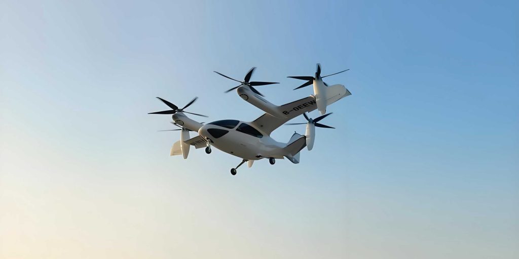
The studied hybrid-wing VTOL drone features four lift-generating rotors mounted on the wings, parallel to the horizontal plane. To minimize adverse aerodynamic interference, the rotors’ centers are positioned near the wing’s aerodynamic center. This VTOL drone operates in three distinct modes:
| Flight Mode | Primary Actuators | Flight Regime |
|---|---|---|
| Rotor Mode | Four Rotors | Hover, Low-Speed Maneuvering |
| Transition Mode | Rotors + Fixed-Wing Surfaces | Acceleration/Deceleration, Mode Switch |
| Fixed-Wing Mode | Fixed-Wing Surfaces & Propeller | High-Speed Cruise |
The transition phase, the focus of control design, involves a coordinated effort where rotor thrust is gradually reduced as aerodynamic forces on the wing and tail build up with increasing forward speed.
1.1 Nonlinear Six-Degree-of-Freedom Model
The equations of motion are derived by considering the combined forces and moments from both the rotor system and the fixed-wing airframe. The translational dynamics in the body frame are given by:
$$ m(\dot{\mathbf{V}}_b + \boldsymbol{\omega} \times \mathbf{V}_b) = \mathbf{f}_b $$
where \( m \) is the mass of the VTOL drone, \( \mathbf{V}_b = [u, v, w]^T \) is the body-axis velocity vector, \( \boldsymbol{\omega} = [p, q, r]^T \) is the angular rate vector, and \( \mathbf{f}_b = [F_x, F_y, F_z]^T \) is the total force vector. Expanding yields:
$$ \begin{aligned}
\dot{u} &= rv – qw + F_x / m \\
\dot{v} &= pw – ru + F_y / m \\
\dot{w} &= qu – pv + F_z / m
\end{aligned} $$
The total forces are the sum of contributions from the fixed-wing (\( \mathbf{F}_f \)) and the rotor system (\( \mathbf{F}_r \)):
$$ \begin{bmatrix} F_x \\ F_y \\ F_z \end{bmatrix} = \begin{bmatrix} F_{fx} \\ F_{fy} \\ F_{fz} \end{bmatrix} + \begin{bmatrix} F_{rx} \\ F_{ry} \\ F_{rz} \end{bmatrix} $$
The rotational dynamics are:
$$ \dot{\boldsymbol{\omega}} = \mathbf{J}^{-1} \left( -\boldsymbol{\omega} \times (\mathbf{J}\boldsymbol{\omega}) + \mathbf{m}_b \right) $$
where \( \mathbf{J} \) is the inertia matrix and \( \mathbf{m}_b = [L, M, N]^T \) is the total moment vector. Similar to forces, the moments are summed:
$$ \begin{bmatrix} L \\ M \\ N \end{bmatrix} = \begin{bmatrix} l_f \\ m_f \\ n_f \end{bmatrix} + \begin{bmatrix} l_r \\ m_r \\ n_r \end{bmatrix} $$
For the longitudinal transition control problem, assuming level flight with no sideslip, the state vector is reduced, and the key longitudinal equations are:
$$ \begin{aligned}
\dot{V} &= \frac{T \cos\alpha – D}{m} – g\sin(\theta – \alpha) \\
\dot{\alpha} &= -\frac{T \sin\alpha + L}{mV} + q + \frac{g}{V}\cos(\theta – \alpha) \\
\dot{q} &= \frac{M}{J_y} \\
\dot{h} &= V\sin(\theta – \alpha) \\
\dot{\theta} &= q
\end{aligned} $$
Here, \( V \) is forward airspeed, \( \alpha \) is angle of attack, \( \theta \) is pitch angle, \( q \) is pitch rate, \( h \) is altitude, \( T \) is fixed-wing thrust, and \( D \) and \( L \) are drag and lift, respectively, which are functions of \( V \), \( \alpha \), and control surface deflections.
1.2 Linear Parameter-Varying (LPV) Model Formulation
The forward airspeed \( V \) is the most significant varying parameter during the transition of the VTOL drone, ranging from 0 m/s (hover) to the minimum fixed-wing cruise speed (e.g., 18 m/s). To facilitate linear control design, an LPV model is constructed. The nonlinear model is trimmed and linearized at multiple operating points across the speed envelope \( V \in [0, 18] \) m/s. The resulting family of linear time-invariant (LTI) models is then parameterized by \( V \), yielding an LPV model:
$$ \begin{aligned}
\dot{\mathbf{x}} &= \mathbf{A}(V)\mathbf{x} + \mathbf{B}(V)\mathbf{u} \\
\mathbf{y} &= \mathbf{C}(V)\mathbf{x}
\end{aligned} $$
where the state vector is \( \mathbf{x} = [V, \alpha, q, h, \theta]^T \), and the control input vector is \( \mathbf{u} = [\delta_t, \delta_e, T_1, T_2]^T \), representing throttle, elevator, and front/rear rotor pair thrusts, respectively. The parameter \( V \) is often normalized for numerical conditioning:
$$ \bar{V} = \frac{V – V_{\text{min}}}{V_{\text{max}} – V_{\text{min}}} $$
The eigenvalue loci of the open-loop LPV system across the speed range reveal the challenge: at low speeds, characteristic roots lie in the right-half plane, indicating instability akin to a multirotor. As speed increases, the roots migrate leftward, reflecting the stabilizing effect of the fixed-wing aerodynamics.
| Speed Regime (V) | Dominant Dynamics | Stability Characteristic |
|---|---|---|
| Low (0-5 m/s) | Rotor-dominated, coupled | Unstable / Marginally Stable |
| Medium (5-12 m/s) | Mixed rotor-wing, highly coupled | Stability varies significantly |
| High (12-18 m/s) | Wing-dominated, aircraft-like | Inherently more stable |
2. Theoretical Foundation: Guardian Maps
Guardian Maps provide a powerful framework for analyzing the generalized stability of parameterized families of matrices or polynomials with respect to a region \( \Omega \) in the complex plane. For a matrix \( \mathbf{A} \), let \( \lambda(\mathbf{A}) \) denote its spectrum. Define the stable set:
$$ S(\Omega) = \{ \mathbf{A} \in \mathbb{R}^{n \times n} : \lambda(\mathbf{A}) \subset \Omega \} $$
A guardian map \( u_{\Omega}(\cdot) \) is a scalar function such that:
$$ u_{\Omega}(\mathbf{A}) = 0 \quad \text{if and only if} \quad \mathbf{A} \in \partial S(\Omega) $$
where \( \partial S(\Omega) \) is the boundary of the stable set. For convex regions relevant to control design, guardian maps can be constructed. Three fundamental regions and their maps are:
1. Left Half-Plane shifted by \( \sigma \): \( \Omega_{\sigma} = \{ s \in \mathbb{C}: \text{Re}(s) < -\sigma \} \).
Guardian Map: \( u_{\sigma}(\mathbf{A}_s) = \det(\mathbf{A}_s \diamond \mathbf{I} – \sigma \mathbf{I} \diamond \mathbf{I}) \det(\mathbf{A}_s – \sigma \mathbf{I}) \), where \( \diamond \) denotes the bialternate product.
2. Disk of radius \( \omega_n \): \( \Omega_{\omega_n} = \{ s \in \mathbb{C}: |s| < \omega_n \} \).
Guardian Map: \( u_{\omega_n}(\mathbf{A}_s) = \det(\mathbf{A}_s \diamond \mathbf{A}_s – \omega_n^2 \mathbf{I} \diamond \mathbf{I}) \det(\mathbf{A}_s^2 – \omega_n^2 \mathbf{I}) \).
3. Cone with damping ratio \( \xi = \cos \theta \): \( \Omega_{\xi} = \{ s \in \mathbb{C}: \text{Re}(s) / |s| < -\xi \} \).
Guardian Map: \( u_{\xi}(\mathbf{A}_s) = \det[\mathbf{A}_s^2 \diamond \mathbf{I} + (1-2\xi^2)\mathbf{A}_s \diamond \mathbf{A}_s] \det(\mathbf{A}_s) \).
A composite desired performance region \( \Omega \) specifying minimum decay rate, maximum natural frequency, and minimum damping ratio can be defined by the guardian map:
$$ u_{\Omega}(\mathbf{A}_s) = u_{\sigma}(\mathbf{A}_s) \cdot u_{\omega_n}(\mathbf{A}_s) \cdot u_{\xi}(\mathbf{A}_s) $$
The key lemma for stability analysis is: Let \( \mathbf{A}(r) \) be a matrix family dependent on a parameter vector \( r \). If there exists some \( r_0 \) such that \( \mathbf{A}(r_0) \) is \( \Omega \)-stable and \( u_{\Omega}(\mathbf{A}(r_0)) \neq 0 \), then the entire family is \( \Omega \)-stable for all \( r \) if and only if \( u_{\Omega}(\mathbf{A}(r_0)) \cdot u_{\Omega}(\mathbf{A}(r)) > 0 \) for all \( r \). This property allows for the automatic determination of the parameter range for which a given controller maintains closed-loop poles within \( \Omega \).
3. Adaptive Switching Controller Design
The control objective for the VTOL drone during transition is to track a commanded airspeed ramp (from 0 to cruise speed) while maintaining altitude. A Linear Quadratic Regulator (LQR) with integral action on tracking error is selected as the baseline control structure for its optimality and robustness properties.
3.1 Controller Structure with Integral Action
Given a trimmed operating point model \( \dot{\mathbf{x}}_0 = \mathbf{A}\mathbf{x}_0 + \mathbf{B}\mathbf{u}, \mathbf{y} = \mathbf{C}\mathbf{x}_0 \), and a reference command \( \mathbf{z} = [V_{cmd}, h_{cmd}]^T \), the tracking error is \( \mathbf{e}_1 = \mathbf{z} – \mathbf{y} \). An integral state \( \mathbf{x}_I = \int \mathbf{e}_1 \, d\tau \) is appended to ensure zero steady-state error. The augmented system is:
$$ \begin{aligned}
\begin{bmatrix} \dot{\mathbf{x}}_0 \\ \dot{\mathbf{x}}_I \end{bmatrix} &=
\begin{bmatrix} \mathbf{A} & \mathbf{0} \\ -\mathbf{C} & \mathbf{0} \end{bmatrix}
\begin{bmatrix} \mathbf{x}_0 \\ \mathbf{x}_I \end{bmatrix} +
\begin{bmatrix} \mathbf{B} \\ \mathbf{0} \end{bmatrix} \mathbf{u} +
\begin{bmatrix} \mathbf{0} \\ \mathbf{I} \end{bmatrix} \mathbf{z} \\
\tilde{\mathbf{e}} &=
\begin{bmatrix} \mathbf{I} \\ \mathbf{0} \end{bmatrix} \mathbf{z} +
\begin{bmatrix} -\mathbf{C} & \mathbf{0} \\ \mathbf{0} & \mathbf{I} \end{bmatrix}
\begin{bmatrix} \mathbf{x}_0 \\ \mathbf{x}_I \end{bmatrix}
\end{aligned} $$
Defining the full state \( \mathbf{X} = [\mathbf{x}_0^T, \mathbf{x}_I^T]^T \), the system becomes \( \dot{\mathbf{X}} = \mathcal{A}\mathbf{X} + \mathcal{B}\mathbf{u} + \mathcal{G}\mathbf{z} \), and the error is \( \tilde{\mathbf{e}} = \mathcal{M}\mathbf{z} + \mathcal{C}_z\mathbf{X} \). The standard LQR cost function is:
$$ J = \frac{1}{2} \int_0^{\infty} \left( \tilde{\mathbf{e}}^T \mathbf{Q} \tilde{\mathbf{e}} + \mathbf{u}^T \mathbf{R} \mathbf{u} \right) dt $$
where \( \mathbf{Q} \succeq 0 \) and \( \mathbf{R} \succ 0 \) are weighting matrices. Minimizing \( J \) leads to the control law:
$$ \mathbf{u} = -\mathbf{K}_x \mathbf{X} – \mathbf{K}_z \mathbf{z} = -\begin{bmatrix} \mathbf{K}_{x0} & \mathbf{K}_{I} \end{bmatrix} \begin{bmatrix} \mathbf{x}_0 \\ \mathbf{x}_I \end{bmatrix} – \mathbf{K}_z \mathbf{z} $$
The gain matrices are computed via the solution \( \mathbf{P} \) of the associated Algebraic Riccati Equation (ARE):
$$ \begin{aligned}
\mathbf{K}_x &= \mathbf{R}^{-1} \mathcal{B}^T \mathbf{P} \\
\mathbf{K}_z &= (\mathbf{P}\mathcal{B}\mathbf{R}^{-1}\mathcal{B}^T – \mathcal{A}^T)^{-1}(\mathcal{C}_z^T\mathbf{Q}\mathcal{M} + \mathbf{P}\mathcal{G})
\end{aligned} $$
3.2 Autonomous Parameter Scheduling via Guardian Maps
The core innovation lies in scheduling the controller gains \( \mathbf{K}_x(V), \mathbf{K}_z(V) \) autonomously using Guardian Maps. The algorithm proceeds as follows:
- Initialization: Design an LQR controller at the transition start condition (e.g., \( V_0 = 0 \) m/s). This yields the initial gain set \( \mathcal{K}_0 \).
- Stability Region Computation: Form the closed-loop matrix \( \mathbf{A}_{cl}(\mathcal{K}_0, V) \) for the LPV system with controller \( \mathcal{K}_0 \) applied. Using the composite guardian map \( u_{\Omega}(\mathbf{A}_{cl}) \), compute the range of the scheduling parameter \( V \) for which \( u_{\Omega}(\mathbf{A}_{cl}(\mathcal{K}_0, V)) > 0 \). This defines the stability region \( \mathcal{V}_0 = [V_{min}, V_{0}^{max}] \) for controller \( \mathcal{K}_0 \).
- Iterative Expansion: Set the next design point at the boundary of the previous stability region, e.g., \( V_1 = V_{0}^{max} \). Compute a new LQR controller \( \mathcal{K}_1 \) for the linearized model at \( V_1 \). Determine its stability region \( \mathcal{V}_1 \). Repeat this process until the union of stability regions \( \bigcup \mathcal{V}_i \) covers the entire transition envelope \( [0, V_{cruise}] \).
- Gain Smoothing: The sequence of gain sets \( \{ \mathcal{K}_0, \mathcal{K}_1, …, \mathcal{K}_N \} \) is obtained. To prevent discontinuous control signals during switching, the gains are interpolated (e.g., via polynomial or linear interpolation) as functions of \( V \), resulting in smooth, continuously scheduled adaptive control laws \( \mathbf{K}_x(V) \) and \( \mathbf{K}_z(V) \).
This method ensures that for every speed \( V \) in the transition, the active controller (or interpolated gain) guarantees the closed-loop poles of the VTOL drone lie within the performance region \( \Omega \).
4. Simulation Analysis and Results
The nonlinear model of the hybrid-wing VTOL drone and the designed adaptive controller are implemented in a simulation environment. The performance region \( \Omega \) is defined with a minimum decay rate \( \sigma = 0.2 \), a maximum natural frequency \( \omega_n = 5.0 \) rad/s, and a minimum damping ratio \( \xi = 0.5 \).
Following the guardian maps-based algorithm, three controller nodes were sufficient to cover the 0-18 m/s envelope. The stability boundaries for each were found autonomously.
| Controller Node | Design Speed (V) | Computed Stable Range (V) |
|---|---|---|
| \( \mathcal{K}_0 \) | 0.0 m/s | [0.0, 0.414] m/s |
| \( \mathcal{K}_1 \) | 0.414 m/s | [0.0, 1.823] m/s |
| \( \mathcal{K}_2 \) | 1.823 m/s | [0.0, >20.56] m/s |
The final scheduled control law was tested on the high-fidelity nonlinear model. The VTOL drone was commanded to accelerate from hover (\( V=0 \), \( h=100m \)) to \( V=18 \) m/s via a ramp command while maintaining altitude.
The simulation results demonstrated the effectiveness of the adaptive control system for the VTOL drone:
- Tracking Performance: The forward speed tracked the commanded ramp accurately and smoothly. Altitude deviation was minimal (less than 0.1 m drop during acceleration) and quickly recovered, showcasing precise energy management.
- Robustness: Additional tests from various initial speeds within the envelope (e.g., 5 m/s, 10 m/s) with step speed commands showed consistent and stable tracking responses, confirming the controller’s robustness across the entire transition regime of the VTOL drone.
- Control Activity: All control inputs—throttle, elevator, and rotor thrusts—varied smoothly and remained within practical saturation limits. The controller automatically coordinated the reduction of rotor thrust as fixed-wing lift increased.
Comparatively, the guardian maps-based adaptive law provided faster speed tracking and better altitude holding with less oscillation than a conventional gain-scheduled controller designed at fixed, sparse operating points without stability region guarantees.
5. Conclusion
This article presented a comprehensive methodology for designing an adaptive switching controller for the critical transition phase of a hybrid-wing VTOL drone. The approach addresses the core challenges of severe parameter variation and dynamic coupling inherent to this flight regime. Key contributions include:
- The development of an integrated nonlinear dynamic model and a corresponding LPV model for the hybrid-wing VTOL drone, accurately capturing its behavior across the speed envelope.
- The application of Guardian Maps theory to autonomously determine the stability regions of candidate controllers in the parameter space. This provides a formal guarantee that the closed-loop poles of the VTOL drone remain within a desired performance region.
- The formulation of an iterative algorithm that automatically synthesizes and schedules LQR-based control gains, ensuring robust stability and performance throughout the entire transition.
Simulation results validate that the proposed adaptive control law enables stable, precise, and coordinated altitude-hold acceleration for the VTOL drone, successfully bridging the gap between rotary-wing and fixed-wing flight modes. The guardian maps-based framework offers a systematic, offline tuning method that significantly reduces the traditional trial-and-error effort associated with gain scheduling for complex systems like the transitioning VTOL drone. Future work will focus on flight testing, extending the strategy to full six-degree-of-flight control including lateral-directional maneuvers, and integrating real-time parameter estimation for enhanced adaptability.