The evolution of unmanned aerial vehicles (UAVs) has been significantly shaped by the demand for versatile platforms capable of operating in constrained environments. Among these, Vertical Take-Off and Landing (VTOL) drones represent a critical technology, merging the hover capability of rotorcraft with the efficient forward flight of fixed-wing aircraft. This article presents a comprehensive study on the dynamics modeling and control of a novel VTOL drone concept. We begin by deriving a complete six-degree-of-freedom (6-DOF) nonlinear mathematical model. Subsequently, we design a robust flight control system based on the Global Fast Terminal Sliding Mode Control (GFTSMC) method for precise altitude and attitude regulation. Comparative simulation results against conventional PID and standard sliding mode controllers demonstrate the superior performance of the proposed approach in terms of precision, convergence speed, and robustness to disturbances.
The operational flexibility of VTOL drones makes them indispensable for modern applications such as precision agriculture, infrastructure inspection, logistics, and surveillance, where runways are unavailable. The core challenge in VTOL drone design lies in managing the complex dynamics during hover, transition, and cruise phases. A robust and accurate mathematical model is the foundational step for developing effective control strategies that ensure stability and performance across all flight regimes. This work focuses on a new drone architecture that utilizes a synergistic combination of tilting and fixed ducted fans to achieve full actuation control during VTOL operations, eliminating the need for traditional aerodynamic control surfaces in hover mode.
Conceptual Design of the Novel VTOL Drone
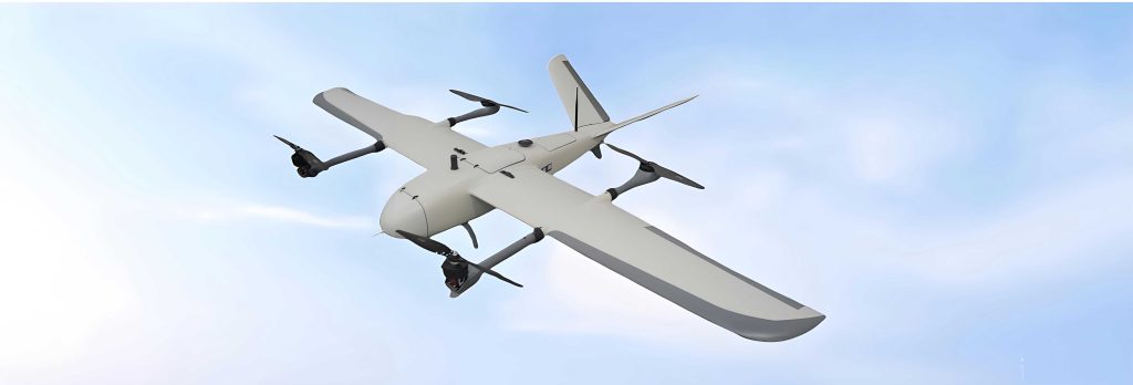
The VTOL drone under investigation features a blended-wing-body fuselage designed for aerodynamic efficiency. The primary lift and control forces during vertical flight and hover are generated by four ducted fans. Two of these fans are mounted on tilting mechanisms at the wingtips, while the other two are fixed, buried within the fuselage at the front and rear. This configuration provides direct control over thrust vectoring. A central payload bay is integrated into the fuselage, equipped with adjustable clamps for secure cargo transportation. The elimination of a tail and rudder surfaces simplifies the structure and reduces drag, relying entirely on differential thrust and thrust vectoring for attitude control.
Six-Degree-of-Freedom Mathematical Modeling
To simulate and control the VTOL drone, a high-fidelity nonlinear mathematical model is essential. The following assumptions are made to facilitate the modeling process while maintaining representative fidelity: 1) The drone and its components are rigid bodies. 2) The total mass and center of gravity (CG) position remain constant. 3) The products of inertia are negligible (assumed zero). 4) The earth is considered an inertial reference frame and flat. 5) Gravitational acceleration and atmospheric density are constant.
Coordinate Systems and Notation
Three primary coordinate frames are used: the Earth-Fixed Inertial Frame (E-frame), the Body-Fixed Frame (B-frame) attached to the drone’s CG, and the Wind/Aerodynamic Frame (W-frame). Transformations between these frames are achieved using rotation matrices based on Euler angles: roll ($\phi$), pitch ($\theta$), and yaw ($\psi$).
Forces and Moments
The total forces and moments acting on the VTOL drone are the sum of contributions from propulsion and aerodynamics.
Propulsive Forces and Moments: The thrust generated by each ducted fan is a primary control input. Let $T_L$ and $T_R$ be the thrust magnitudes of the left and right tilting ducted fans, with tilt angles $\theta_{TL}$ and $\theta_{TR}$, respectively. Let $T_{F1}$ and $T_{F2}$ be the thrust magnitudes of the front and rear fixed ducted fans. The total thrust vector in the body frame is:
$$
\begin{aligned}
T_x &= T_L \cos\theta_{TL} + T_R \cos\theta_{TR} \\
T_y &= 0 \\
T_z &= T_L \sin\theta_{TL} + T_R \sin\theta_{TR} + T_{F1} + T_{F2}
\end{aligned}
$$
The corresponding moments generated by these forces about the CG are:
$$
\begin{aligned}
l_p &= (T_L \sin\theta_{TL} – T_R \sin\theta_{TR}) \cdot L_T \\
m_p &= (T_{F1} – T_{F2}) \cdot L_F \\
n_p &= (T_L – T_R) \cdot L_T
\end{aligned}
$$
where $L_T$ is the lateral arm from the CG to the wingtip fans, and $L_F$ is the longitudinal arm from the CG to the front/rear fans.
Aerodynamic Forces and Moments: During forward flight, the blended-wing-body generates aerodynamic forces. These are expressed in the wind frame and then transformed to the body frame. The aerodynamic force vector $[D, Y, L]^T$ (Drag, Sideforce, Lift) and moment vector $[l_a, m_a, n_a]^T$ (rolling, pitching, yawing) are given by:
$$
\begin{aligned}
D = C_D \bar{q} S, \quad & Y = C_Y \bar{q} S, \quad & L = C_L \bar{q} S \\
l_a = C_l \bar{q} S b, \quad & m_a = C_m \bar{q} S \bar{c}, \quad & n_a = C_n \bar{q} S b
\end{aligned}
$$
where $C_*$ are the non-dimensional force and moment coefficients, $\bar{q} = \frac{1}{2} \rho V^2$ is the dynamic pressure, $S$ is the wing reference area, $b$ is the wingspan, and $\bar{c}$ is the mean aerodynamic chord.
Equations of Motion
Translational Dynamics (in Earth Frame): Applying Newton’s second law and resolving forces into the Earth frame yields:
$$
m
\begin{bmatrix}
\dot{V}_{xg} \\ \dot{V}_{yg} \\ \dot{V}_{zg}
\end{bmatrix}
= L_g^b
\begin{bmatrix}
T_x \\ T_y \\ -T_z
\end{bmatrix}
+ L_g^a
\begin{bmatrix}
-D \\ Y \\ -L
\end{bmatrix}
+
\begin{bmatrix}
0 \\ 0 \\ mg
\end{bmatrix}
$$
Here, $m$ is the mass, $[V_{xg}, V_{yg}, V_{zg}]^T$ is the velocity vector in the Earth frame, $g$ is gravity, and $L_g^b$ and $L_g^a$ are transformation matrices from the body and wind frames to the Earth frame, respectively.
$$
L_g^b = \begin{bmatrix}
c\theta c\psi & c\theta s\psi & -s\theta \\
-c\phi s\psi + s\phi s\theta c\psi & c\phi c\psi + s\phi s\theta s\psi & s\phi c\theta \\
s\phi s\psi + c\phi s\theta c\psi & -s\phi c\psi + c\phi s\theta s\psi & c\phi c\theta
\end{bmatrix}
$$
where $s\cdot$ and $c\cdot$ denote $\sin(\cdot)$ and $\cos(\cdot)$.
Rotational Dynamics (in Body Frame): The rotational dynamics are derived from Euler’s moment equation:
$$
\begin{aligned}
\dot{p} &= I_x^{-1}[(I_y – I_z)qr + l_a + l_p] \\
\dot{q} &= I_y^{-1}[(I_z – I_x)pr + m_a + m_p] \\
\dot{r} &= I_z^{-1}[(I_x – I_y)pq + n_a + n_p]
\end{aligned}
$$
where $[p, q, r]^T$ is the angular velocity vector in the body frame, and $I_x, I_y, I_z$ are the moments of inertia.
Kinematic Equations: The relationship between Euler angle rates and body angular rates is:
$$
\begin{bmatrix} \dot{\phi} \\ \dot{\theta} \\ \dot{\psi} \end{bmatrix} =
\begin{bmatrix}
1 & \sin\phi \tan\theta & \cos\phi \tan\theta \\
0 & \cos\phi & -\sin\phi \\
0 & \sin\phi \sec\theta & \cos\phi \sec\theta
\end{bmatrix}
\begin{bmatrix} p \\ q \\ r \end{bmatrix}
$$
The navigation equations and relationships between airspeed ($V$), angle of attack ($\alpha$), and sideslip ($\beta$) are also defined but omitted here for brevity. This complete set of equations forms the nonlinear model implemented in a simulation environment like MATLAB/Simulink for analysis and controller design.
Controller Design Using Global Fast Terminal Sliding Mode Control
Precise control of altitude and attitude is paramount for the stable operation of a VTOL drone, especially during take-off, landing, and hover. Sliding Mode Control (SMC) is renowned for its robustness against model uncertainties and external disturbances. To achieve finite-time convergence and fast dynamic response, we employ the Global Fast Terminal Sliding Mode Control (GFTSMC) method.
Principles of GFTSMC
Consider a second-order uncertain system:
$$
\ddot{x} = f(x, \dot{x}) + g(x, \dot{x}) u + d(t)
$$
where $|d(t)| \le L$ represents bounded disturbances/uncertainties. The control objective is to track a desired trajectory $x_d(t)$.
First, define a global fast terminal sliding surface $s$:
$$
s = \dot{e} + a e + b e^{q/p}
$$
where $e = x_d – x$ is the tracking error, $a, b > 0$, and $p, q$ are positive odd integers satisfying $p > q$. This surface guarantees that once $s=0$, the error dynamics $\dot{e} = -a e – b e^{q/p}$ converge to zero in finite time $t_s$:
$$
t_s = \frac{p}{a(p-q)} \ln\left( \frac{a e(0)^{(p-q)/p} + b}{b} \right)
$$
The control law $u$ is designed to drive the system to this surface. It typically consists of an equivalent control $u_{eq}$ (based on the nominal model) and a switching/discontinuous control $u_{sw}$ to reject disturbances:
$$
u = g^{-1} \left[ \ddot{x}_d – f + a \dot{e} + b \frac{q}{p} e^{(q/p)-1} \dot{e} + \rho s + \lambda \text{sgn}(s) \right]
$$
where $\rho, \lambda > 0$, and $\lambda \ge L$. The $\text{sgn}(s)$ term ensures attraction to the sliding manifold.
Application to VTOL Drone Control
We design separate GFTSMC controllers for altitude ($z$), roll ($\phi$), pitch ($\theta$), and yaw ($\psi$). Each channel is treated as a second-order system based on the derived dynamics.
1. Roll Angle ($\phi$) Controller:
Let $x_1 = \phi$, $x_2 = \dot{\phi} = p$. From the rotational dynamics:
$$
\ddot{\phi} \approx \dot{p} = \frac{I_y – I_z}{I_x} q r + \frac{1}{I_x} u_\phi + d_\phi(t)
$$
where $u_\phi$ is the virtual control input (rolling moment generated by differential thrust). The sliding surface is:
$$
s_\phi = \dot{e}_\phi + a_\phi e_\phi + b_\phi e_\phi^{q_\phi/p_\phi}, \quad e_\phi = \phi_d – \phi
$$
The GFTSMC law for the roll channel is:
$$
\begin{aligned}
u_\phi = I_x \Bigg[ \ddot{\phi}_d &- \frac{I_y – I_z}{I_x} q r + a_\phi \dot{e}_\phi + b_\phi \frac{q_\phi}{p_\phi} e_\phi^{(q_\phi/p_\phi)-1} \dot{e}_\phi \\
&+ \rho_\phi s_\phi + \lambda_\phi \text{sgn}(s_\phi) \Bigg]
\end{aligned}
$$
2. Pitch Angle ($\theta$) Controller:
Similarly, based on $\ddot{\theta} \approx \dot{q}$:
$$
u_\theta = I_y \left[ \ddot{\theta}_d – \frac{I_z – I_x}{I_y} p r + a_\theta \dot{e}_\theta + b_\theta \frac{q_\theta}{p_\theta} e_\theta^{(q_\theta/p_\theta)-1} \dot{e}_\theta + \rho_\theta s_\theta + \lambda_\theta \text{sgn}(s_\theta) \right]
$$
3. Yaw Angle ($\psi$) Controller:
Based on $\ddot{\psi} \approx \dot{r}$:
$$
u_\psi = I_z \left[ \ddot{\psi}_d – \frac{I_x – I_y}{I_z} p q + a_\psi \dot{e}_\psi + b_\psi \frac{q_\psi}{p_\psi} e_\psi^{(q_\psi/p_\psi)-1} \dot{e}_\psi + \rho_\psi s_\psi + \lambda_\psi \text{sgn}(s_\psi) \right]
$$
4. Altitude ($z$) Controller:
The vertical dynamics from the translational equation, assuming small angles during hover, simplify to:
$$
\ddot{z} = \frac{T_z}{m} \cos\phi \cos\theta – g + d_z(t)
$$
where $T_z$ is the total vertical thrust (the sum of all fan contributions projected vertically). The control law for the total vertical thrust command is:
$$
u_z = m \left[ \ddot{z}_d + g + a_z \dot{e}_z + b_z \frac{q_z}{p_z} e_z^{(q_z/p_z)-1} \dot{e}_z + \rho_z s_z + \lambda_z \text{sgn}(s_z) \right] / (\cos\phi \cos\theta)
$$
where $e_z = z_d – z$.
These virtual control inputs ($u_\phi, u_\theta, u_\psi, u_z$) are then mapped to the actual actuator commands (individual fan thrusts $T_L, T_R, T_{F1}, T_{F2}$ and tilt angles $\theta_{TL}, \theta_{TR}$) through a control allocation scheme, which solves for the actuator settings that produce the desired net forces and moments.
Comparative Controller Designs
To benchmark the performance of the GFTSMC, we also design two other controllers for comparison:
1. Conventional PID Controller: The standard linear controller with proportional, integral, and derivative terms.
$$
u_{PID} = K_p e + K_i \int e \, dt + K_d \dot{e}
$$
2. Linear Sliding Mode Controller (LSMC): Uses a linear sliding surface $s = \dot{e} + \nu e$ with an exponential reaching law $ \dot{s} = -k s – \eta \, \text{sgn}(s)$.
$$
u_{LSMC} = g^{-1} \left[ \ddot{x}_d – f + \nu \dot{e} + k s + \eta \, \text{sgn}(s) \right]
$$
The following table summarizes the key controller parameters used in the simulation.
| Controller Type | Controlled Variable | Key Parameters |
|---|---|---|
| GFTSMC | Roll ($\phi$) | $a_\phi=2, b_\phi=1, p_\phi=9, q_\phi=5, \rho_\phi=100, \lambda_\phi=3.0$ |
| Pitch ($\theta$) | $a_\theta=2, b_\theta=1, p_\theta=9, q_\theta=5, \rho_\theta=100, \lambda_\theta=3.0$ | |
| Yaw ($\psi$) | $a_\psi=2, b_\psi=1, p_\psi=9, q_\psi=5, \rho_\psi=100, \lambda_\psi=3.0$ | |
| Altitude ($z$) | $a_z=2, b_z=1, p_z=9, q_z=5, \rho_z=100, \lambda_z=3.0$ | |
| LSMC | Roll ($\phi$) | $\nu_\phi=5, k_\phi=2, \eta_\phi=0.01$ |
| Pitch ($\theta$) | $\nu_\theta=5, k_\theta=2, \eta_\theta=0.01$ | |
| Yaw ($\psi$) | $\nu_\psi=5, k_\psi=2, \eta_\psi=0.01$ | |
| Altitude ($z$) | $\nu_z=5, k_z=2, \eta_z=0.01$ | |
| PID | Roll/Pitch/Yaw | $K_p=2, K_i=2, K_d=0$ |
| Altitude ($z$) | $K_p=5, K_i=2, K_d=1$ |
Simulation Results and Performance Analysis
A high-fidelity simulation model of the VTOL drone was constructed in MATLAB/Simulink based on the derived nonlinear equations. The simulation scenario involves a hover stabilization and maneuver task. The VTOL drone starts from an initial hover at 10 m altitude with zero orientation angles. At time t=0, step commands are issued: altitude $z_d = 20$ m, roll angle $\phi_d = 10^\circ$, pitch angle $\theta_d = 10^\circ$, and yaw angle $\psi_d = 10^\circ$. To evaluate robustness, a sinusoidal disturbance $d(t) = 2\sin(t)$ is injected into each channel’s dynamics. The physical parameters of the drone model are: mass $m = 5$ kg, moments of inertia $I_x = 0.1755\, \text{kg·m}^2$, $I_y = 0.1396\, \text{kg·m}^2$, $I_z = 0.243\, \text{kg·m}^2$, and $g = 9.8\, \text{m/s}^2$.
The performance metrics analyzed include: Settling Time (time to reach and stay within 2% of the final command), Overshoot (%), and Steady-State Error. The comparative results are summarized below.
| Control Variable | Controller | Settling Time (s) | Overshoot (%) | Steady-State Error | Remarks |
|---|---|---|---|---|---|
| Altitude (z) | GFTSMC | ~2.1 | 0 | Negligible | Fast, precise, no overshoot. |
| LSMC | ~3.5 | ~1.5 | Small chattering | Slower, slight chattering. | |
| PID | >5.0 | >15 | Small | Significant initial drop (“drop-out”), large overshoot. | |
| Roll Angle (φ) | GFTSMC | ~1.8 | 0 | Negligible | Finite-time convergence, robust. |
| LSMC | ~2.5 | ~2 | Minor chattering | Good but slower than GFTSMC. | |
| PID | ~3.0 | ~8 | Negligible | Clear overshoot and slower settling. | |
| Pitch Angle (θ) | GFTSMC | ~1.8 | 0 | Negligible | Performance identical to roll channel. |
| LSMC | ~2.5 | ~2 | Minor chattering | Consistent with roll channel behavior. | |
| PID | ~3.0 | ~8 | Negligible | Consistent overshoot issue. | |
| Yaw Angle (ψ) | GFTSMC | ~2.0 | 0 | Negligible | Fast and precise yaw control. |
| LSMC | ~2.8 | ~1.5 | Minor chattering | Acceptable but slower response. | |
| PID | ~3.5 | ~6 | Negligible | Overshoot present, slowest settling. |
Key Observations from Simulation:
- Superiority of GFTSMC: The Global Fast Terminal Sliding Mode Controller consistently outperforms both the Linear SMC and PID controllers. It achieves the fastest settling time for all four controlled variables with zero overshoot. This is a direct consequence of its finite-time convergence property encoded in the terminal sliding surface.
- Robustness: All sliding mode controllers (GFTSMC and LSMC) effectively reject the applied sinusoidal disturbance $d(t)=2\sin(t)$, maintaining tight tracking. The GFTSMC does this with less observable chattering in the control input compared to the standard LSMC, thanks to its faster convergence reducing the time spent in the reaching phase.
- PID Limitations: The conventional PID controller, while stable, exhibits significant shortcomings. It shows considerable overshoot in the attitude angles (6-15%) and a particularly problematic “drop-out” or loss of altitude during the initial aggressive maneuver to achieve the new attitude commands. This highlights its lack of inherent robustness and poor handling of strongly coupled nonlinear dynamics, which are characteristic of this type of VTOL drone.
- Control Effort: Analysis of the control inputs (thrust and moment commands) shows that the GFTSMC provides smooth yet aggressive initial control action to achieve fast convergence, which quickly settles to a steady-state value. The LSMC shows higher-frequency activity (chattering) due to the signum function, and the PID controller shows a slower, more oscillatory control effort corresponding to its output response.
The simulation validates that the derived nonlinear model accurately captures the dynamics of the novel VTOL drone and that the proposed GFTSMC is a highly effective control solution, offering a superior blend of speed, precision, and robustness essential for reliable autonomous flight.
Conclusion
This article presented a detailed framework for the modeling and control of a novel VTOL drone architecture. A complete six-degree-of-freedom nonlinear mathematical model was rigorously derived, encompassing the unique propulsion system combining tilting and fixed ducted fans. This model serves as a critical tool for simulation and analysis. To address the critical need for precise and robust control during hover and low-speed flight, a Global Fast Terminal Sliding Mode Control (GFTSMC) strategy was designed for altitude and attitude regulation. The GFTSMC law was specifically developed to guarantee finite-time convergence and excellent disturbance rejection. Through comparative numerical simulations with a Linear Sliding Mode Controller and a conventional PID controller, the GFTSMC demonstrated unequivocal superiority. It achieved faster settling times, eliminated overshoot, and maintained robust performance in the presence of external disturbances, with minimal control chattering. These results confirm that the GFTSMC is a powerful and suitable control methodology for stabilizing and maneuvering the complex, nonlinear system represented by this advanced VTOL drone, paving the way for reliable implementation in real-world applications.