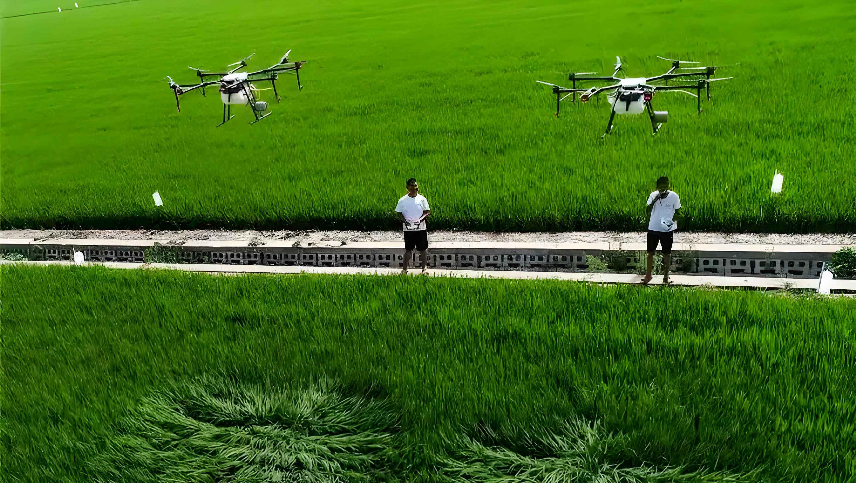
With the rapid advancement of unmanned aerial vehicle technology, its application in agriculture has garnered significant attention, particularly in optimizing efficient operational strategies. In crop spraying operations, spraying UAVs face dual constraints of battery capacity and pesticide tank volume, which often prevent a single flight from covering entire fields. To address this, we introduce a multi-trip operation mode, where crop spraying drones can return to supply stations for recharging and refilling, enabling multiple spraying trips. This paper focuses on the path optimization problem for crop spraying drones under these practical constraints, aiming to minimize operational costs by integrating spraying sequence optimization, flight path planning, and multi-drone scheduling.
We formulate an integer linear programming model that captures the essence of the problem. Consider a directed graph $$G = (N, A)$$, where $$N$$ is the set of nodes including the depot (node 0), spraying task nodes $$N_t$$, and a supply station (node $$s$$). The arc set $$A$$ represents connections between nodes, with associated energy consumption $$e_{ij}$$ and travel time $$t_{ij}$$. The task arc set $$A_t \subseteq A$$ requires spraying, with each arc $$(i,j) \in A_t$$ having a positive spraying demand $$d_{ij}$$. A homogeneous fleet of crop spraying drones $$K$$ is available, each equipped with a battery capacity $$B$$ and a pesticide tank capacity $$Q$$. The objective is to minimize the total cost, comprising travel cost, fixed drone usage cost, and service cost at the supply station.
The ILP model is defined as follows. The decision variables include: $$x_{ijk}^m$$, an integer variable indicating the number of times drone $$k$$ traverses arc $$(i,j)$$ during trip $$m$$; $$y_{ijk}^m$$, a binary variable equal to 1 if drone $$k$$ sprays arc $$(i,j)$$ during trip $$m$$, 0 otherwise; $$z_k^m$$, a binary variable equal to 1 if drone $$k$$ executes spraying trip $$m$$, 0 otherwise; and $$u_{ik}^m$$, an integer variable representing the visiting sequence of node $$i$$ by drone $$k$$ during trip $$m$$. The objective function is:
$$ \min \sum_{k \in K} \sum_{m \in M_k} \left( \sum_{(i,j) \in A} c_{ij} x_{ijk}^m + f z_k^m + g \delta_k^m \right) $$
where $$c_{ij}$$ is the unit travel cost, $$f$$ is the fixed cost per drone, $$g$$ is the service cost at the supply station, and $$\delta_k^m$$ indicates if drone $$k$$ visits the supply station in trip $$m$$. Subject to constraints such as flow conservation:
$$ \sum_{j \in N} x_{ijk}^m – \sum_{j \in N} x_{jik}^m = 0 \quad \forall i \in N \setminus \{0,s\}, k \in K, m \in M_k $$
Spraying coverage for each task arc:
$$ \sum_{k \in K} \sum_{m \in M_k} y_{ijk}^m = 1 \quad \forall (i,j) \in A_t $$
Battery and tank capacity limits per trip:
$$ \sum_{(i,j) \in A} e_{ij} x_{ijk}^m \leq B \quad \forall k \in K, m \in M_k $$
$$ \sum_{(i,j) \in A_t} d_{ij} y_{ijk}^m \leq Q \quad \forall k \in K, m \in M_k $$
And sub-tour elimination constraints:
$$ u_{ik}^m – u_{jk}^m + L x_{ijk}^m \leq L – 1 \quad \forall i,j \in N, k \in K, m \in M_k $$
This model efficiently integrates the multi-trip aspect, ensuring that spraying UAVs can operate within their physical limits while optimizing the overall cost.
To solve this complex combinatorial optimization problem, we propose an improved Adaptive Large Neighborhood Search algorithm. The ALNS framework is chosen for its ability to dynamically adjust operator selection based on historical performance, enhancing solution quality. Our algorithm starts with an initial feasible solution generated using a sequence-based method, where spraying tasks are ordered by the smallest node index and assigned to drones greedily. The ALNS iteratively destroys and repairs the current solution using a set of removal and insertion operators, with an embedded Simulated Annealing mechanism for accepting worse solutions to escape local optima.
We design four removal operators and three insertion operators tailored to the crop spraying drone problem. The removal operators include: Random Removal, which randomly selects tasks to remove; Trip Removal, which removes all tasks from a randomly chosen trip; Highest Cost Removal, which removes tasks with the highest marginal cost defined as $$\Delta cost = C – C_{-task}$$, where $$C$$ is the current trip cost and $$C_{-task}$$ is the cost after removal; and Shaw Removal, which removes tasks based on similarity measured by:
$$ \phi(i,j) = \alpha \cdot dist(i,j) + \beta \cdot |t_i – t_j| + \gamma \cdot |dur_i – dur_j| $$
with weights $$\alpha=1.0$$, $$\beta=0.5$$, $$\gamma=0.2$$. The insertion operators include: Random Insertion, which inserts tasks randomly into feasible positions; Greedy Insertion, which inserts tasks at the position with the lowest marginal cost $$\Delta cost = C_{+task} – C$$; and Regret Insertion, which prioritizes tasks with the highest regret value, defined as the difference between the best and second-best insertion costs.
The adaptive mechanism updates operator weights periodically based on scores. Let $$\sigma_r$$ and $$\sigma_i$$ be the scores for removal and insertion operators, with weights $$\omega_r$$ and $$\omega_i$$. The probability of selecting operator $$r$$ is:
$$ P_r = \frac{\omega_r}{\sum_{r’ \in R} \omega_{r’}} $$
Weights are updated as $$\omega_r = \omega_r (1-\rho) + \rho \frac{\sigma_r}{n_r}$$, where $$\rho=0.4$$ is the reaction factor, and $$n_r$$ is the number of times operator $$r$$ was used. Scores are increased by $$\theta_1=20$$ for new global best solutions, $$\theta_2=10$$ for improved solutions, and $$\theta_3=3$$ for accepted worse solutions. The SA acceptance probability is $$P(accept) = \exp\left( \frac{-(C_{new} – C_{current})}{T} \right)$$, with initial temperature $$T_0=100$$ and cooling rate $$\alpha_c=0.9$$. The algorithm terminates after a maximum number of iterations (1000 for small instances, 2000 for medium, 5000 for large) or no improvement for a set number of iterations.
We conduct numerical experiments to validate the model and algorithm. Instances of varying sizes are generated, with nodes ranging from 12 to 62 and spraying task arcs from 5 to 30. Key parameters include tank capacity $$Q=50$$, battery capacity $$B$$ from 150 to 400, and maximum operation time $$T_{max}$$ from 12 to 24. Travel costs $$c_{ij}$$, fixed costs $$f$$, and service costs $$g$$ are randomly generated within specified ranges. Pre-experiments determine optimal parameters for the ALNS, leading to the selection of $$\theta_1=20$$, $$\theta_2=10$$, $$\theta_3=3$$, and $$\alpha_c=0.9$$.
| Instance Group | Number of Nodes | Number of Spraying Task Arcs | Q | B | T_max |
|---|---|---|---|---|---|
| ISG1 | 12 | 5 | 50 | 150 | 12 |
| ISG2 | 16 | 7 | 50 | 150 | 12 |
| ISG3 | 20 | 9 | 50 | 150 | 12 |
| ISG4 | 22 | 10 | 50 | 150 | 12 |
| ISG5 | 24 | 11 | 50 | 150 | 12 |
| ISG6 | 28 | 13 | 50 | 150 | 12 |
| ISG7 | 32 | 15 | 50 | 200 | 12 |
| ISG8 | 42 | 20 | 50 | 300 | 24 |
| ISG9 | 52 | 25 | 50 | 300 | 24 |
| ISG10 | 62 | 30 | 50 | 400 | 24 |
We compare our ALNS algorithm with the commercial solver CPLEX and a rule-based sequence generation method (Rule). For small-scale instances (ISG1-ISG3), ALNS consistently finds global optimal solutions, matching CPLEX but with significantly shorter computation times. For medium-scale instances (ISG4-ISG6), ALNS outperforms CPLEX in solution quality, with improvements ranging from 0.79% to 7.18%, and achieves an average runtime of 13.68 seconds compared to CPLEX’s 7200 seconds limit. For large-scale instances (ISG7-ISG10), ALNS demonstrates substantial advantages over the Rule method, with an average improvement of 18.00% in objective function value and an average runtime of 278.55 seconds.
| Instance | GA Objective | GA Time (s) | ACO Objective | ACO Time (s) | ALNS Objective | ALNS Time (s) |
|---|---|---|---|---|---|---|
| ISG1-1 | 481 | 2.48 | 481 | 2.40 | 481 | 2.44 |
| ISG1-2 | 275 | 2.26 | 275 | 2.29 | 275 | 1.32 |
| ISG1-3 | 2135 | 2.43 | 2135 | 2.50 | 2135 | 1.25 |
| ISG2-1 | 408 | 3.13 | 408 | 3.72 | 408 | 2.15 |
| ISG2-2 | 372 | 3.06 | 372 | 3.65 | 372 | 3.45 |
| ISG2-3 | 1047 | 2.96 | 1047 | 3.53 | 1047 | 2.23 |
| ISG3-1 | 1473 | 4.12 | 1473 | 5.30 | 1473 | 8.28 |
| ISG3-2 | 1588 | 4.08 | 1588 | 5.37 | 1588 | 11.40 |
| ISG3-3 | 4264 | 3.95 | 4096 | 5.41 | 4096 | 12.56 |
| ISG4-1 | 1704 | 13.06 | 1556 | 12.22 | 1556 | 8.09 |
| ISG4-2 | 552 | 12.52 | 502 | 12.00 | 470 | 7.53 |
| ISG4-3 | 2820 | 13.63 | 2759 | 12.26 | 2716 | 9.31 |
| ISG5-1 | 1409 | 15.40 | 1404 | 23.78 | 1348 | 11.87 |
| ISG5-2 | 4496 | 13.75 | 4268 | 26.27 | 4088 | 13.94 |
| ISG5-3 | 2948 | 14.94 | 2980 | 24.17 | 2972 | 12.24 |
| ISG6-1 | 5440 | 16.57 | 5340 | 28.19 | 4880 | 23.71 |
| ISG6-2 | 1789 | 16.11 | 1797 | 27.79 | 1694 | 15.76 |
| ISG6-3 | 3178 | 15.84 | 3002 | 27.77 | 2967 | 20.64 |
| ISG7-1 | 8939 | 55.09 | 9211 | 76.89 | 9106 | 39.73 |
| ISG7-2 | 6717 | 48.41 | 6887 | 72.30 | 6697 | 32.34 |
| ISG7-3 | 4274 | 47.63 | 4379 | 71.57 | 4215 | 30.04 |
| ISG8-1 | 7060 | 68.13 | 6586 | 119.20 | 6127 | 120.35 |
| ISG8-2 | 12630 | 68.89 | 10805 | 120.78 | 10351 | 115.61 |
| ISG8-3 | 5532 | 66.94 | 5123 | 120.74 | 4843 | 109.73 |
| ISG9-1 | 6758 | 109.20 | 6484 | 166.72 | 6274 | 201.23 |
| ISG9-2 | 15563 | 108.60 | 14222 | 174.45 | 13188 | 280.32 |
| ISG9-3 | 7811 | 107.98 | 7811 | 167.78 | 7542 | 340.18 |
| ISG10-1 | 16216 | 158.61 | 16435 | 256.71 | 15561 | 832.59 |
| ISG10-2 | 9479 | 153.56 | 8781 | 237.60 | 8350 | 606.80 |
| ISG10-3 | 11288 | 158.53 | 10856 | 241.67 | 10298 | 633.65 |
Furthermore, we compare ALNS with mainstream metaheuristics: Genetic Algorithm and Ant Colony Optimization. For medium-scale instances, ALNS achieves average improvements of 6.90% over GA and 3.55% over ACO. For large-scale instances, the improvements are 7.84% and 4.47%, respectively. These results underscore the effectiveness of our ALNS algorithm in handling the complexities of multi-trip routing for crop spraying drones.
In conclusion, our study addresses the practical challenge of path optimization for spraying UAVs under battery and tank constraints by introducing a multi-trip operation mode and developing an efficient ILP model and ALNS algorithm. The proposed solution significantly reduces operational costs and demonstrates robustness across various instance sizes. Future work could extend to other agricultural operations, such as seeding and remote sensing, incorporate multi-objective optimization, consider heterogeneous drone fleets, and account for uncertainties in flight time and pesticide consumption. Additionally, integrating minimum turning radius constraints and robust optimization techniques would enhance the practicality and resilience of drone operations in dynamic agricultural environments.