
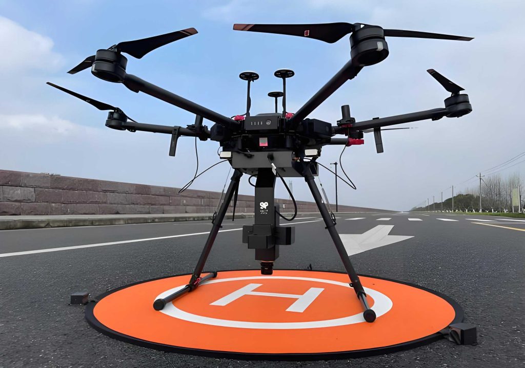
I study the design, optimization, and real-world deployment of a deep learning based target tracking system for quadrotor UAV drones. In my work, UAV drones are not treated as simple flying cameras. They are treated as mobile edge computing platforms that must perceive a target, estimate its position, maintain a stable flight attitude, and execute tracking under strict limits on power, weight, memory, and computation. This combination of computer vision, embedded inference, and flight control creates a challenging engineering problem. I focus on how to make visual tracking accurate enough for complex scenes while remaining fast enough for onboard UAV drones.
1. Research Motivation and System Scope
Target tracking is one of the core capabilities of intelligent UAV drones. It supports aerial photography, security monitoring, autonomous navigation, path planning, and target following. However, the tracking problem on UAV drones differs from ground-based tracking. Ground platforms often have access to stable cameras, desktop GPUs, and relatively predictable backgrounds. UAV drones, by contrast, experience camera motion, viewpoint changes, small target scales, low resolution, motion blur, illumination variation, background clutter, similar objects, partial occlusion, full occlusion, out-of-view events, and rapid scale changes. These challenges are not independent. They often occur together, and a single tracking failure can propagate into a complete loss of the target.
I organize the major tracking challenges for UAV drones in the table below.
| Challenge | Description | Effect on UAV Drone Tracking |
|---|---|---|
| Scale Variation | Target size changes over time. | Box regression becomes unstable, especially during rapid approach or retreat. |
| Aspect Ratio Change | Width and height relationship changes. | Viewpoint changes distort appearance and reduce matching accuracy. |
| Low Resolution | Target contains few pixels. | Deep semantic features are weak, and shallow details become critical. |
| Fast Motion | Target moves quickly across frames. | Search region may not contain the target, causing drift. |
| Full Occlusion | Target is completely hidden. | Tracker must recover after the target reappears. |
| Partial Occlusion | Part of the target is hidden. | Feature matching may lock onto the visible distractor. |
| Out-of-View | Target leaves the image boundary. | Tracker must avoid updating on background. |
| Background Clutter | Background contains confusing patterns. | Classifier may confuse foreground and background. |
| Illumination Variation | Lighting changes across the scene. | Appearance model may become inconsistent. |
| Viewpoint Change | Camera or target orientation changes. | Template and search features become misaligned. |
| Camera Motion | The UAV drone camera moves abruptly. | Global motion is mixed with target motion. |
| Similar Object | Distractors look like the target. | Peak response may move to the wrong object. |
For UAV drones, a usable tracker must balance accuracy and latency. A high-accuracy model that runs at two frames per second is not useful for closed-loop flight. A very fast model that loses the target after one occlusion is also not useful. Therefore, I define the design objective as a multi-objective optimization problem. I want to minimize model parameters, computation, and latency while maximizing tracking success, precision, and robustness. I summarize the main evaluation metrics used in my work below.
| Metric | Meaning | Preferred Direction |
|---|---|---|
| IoU | Intersection over union between predicted and ground-truth boxes. | Higher |
| AUC | Area under the success curve over IoU thresholds. | Higher |
| Precision | Fraction of frames whose center error is below a threshold. | Higher |
| AO | Average overlap across all frames in a test set. | Higher |
| SR0.5 | Fraction of frames with IoU greater than 0.5. | Higher |
| SR0.75 | Fraction of frames with IoU greater than 0.75. | Higher |
| Parameters | Number of learnable weights. | Lower |
| Computation | Floating-point operations or equivalent workload. | Lower |
| FPS | Frames processed per second. | Higher |
The core geometric metric is intersection over union. I use it throughout my evaluation because it jointly reflects localization and scale estimation:
$$IoU = \frac{|B_{pred} \cap B_{gt}|}{|B_{pred} \cup B_{gt}|}$$
For center-based precision, I measure the Euclidean distance between the predicted center and the ground-truth center:
$$Error = \sqrt{(\hat{x}-x)^2+(\hat{y}-y)^2}$$
For long-term benchmarks, average overlap is computed over all frames:
$$AO = \frac{1}{N}\sum_{i=1}^{N} IoU_i$$
The success rate at a threshold is defined as:
$$SR_t = \frac{N_{IoU>t}}{N}$$
These metrics guide every design choice in my system. I do not optimize only for accuracy on a GPU. I optimize for a complete UAV drone tracking pipeline that can run on embedded hardware while preserving enough precision for practical missions.
2. Deep Learning Foundations for UAV Drone Tracking
My tracker is built on two deep learning families: convolutional neural networks and Transformer networks. Convolutional neural networks provide efficient local feature extraction and strong inductive bias. Transformer networks provide global context modeling and flexible attention based interaction. For UAV drones, neither family alone is sufficient. Pure convolutional trackers are fast but may lack global reasoning. Pure Transformer trackers are accurate but often too heavy for onboard inference. I therefore combine them.
A standard convolution layer computes a weighted sum over a local receptive field:
$$Y(i,j)=\sum_{m=1}^{k}\sum_{n=1}^{k}X(i+m-1,j+n-1)W(m,n)+b$$
Max pooling selects the strongest local response:
$$Y(i,j)=\max_{m,n \in R} X(i\cdot s+m, j\cdot s+n)$$
Average pooling smooths local responses:
$$Y(i,j)=\frac{1}{k^2}\sum_{m=1}^{k}\sum_{n=1}^{k}X(i\cdot s+m, j\cdot s+n)$$
A fully connected layer maps features to an output space:
$$y = Wx+b$$
These operations are efficient, but convolution alone has limitations for UAV drone tracking. The receptive field grows gradually, and long-range dependencies between the target and the search region are not modeled directly. Transformer attention addresses this issue. Scaled dot-product attention is defined as:
$$Attention(Q,K,V)=softmax\left(\frac{QK^T}{\sqrt{d_k}}\right)V$$
A Vision Transformer encoder layer consists of multi-head self-attention, normalization, and a multi-layer perceptron:
$$z’_l = MSA(LN(z_{l-1}))+z_{l-1}$$
$$z_l = MLP(LN(z’_l))+z’_l$$
The computational cost of multi-head attention is a central concern for UAV drones. For an input feature map with height H, width W, and channel dimension C, the standard multi-head attention cost can be expressed as:
$$\Omega(MHA)=4HWC^2+2(HW)^2C$$
This cost grows quadratically with the number of spatial tokens. On a desktop GPU, this may be acceptable. On a UAV drone powered by an embedded NPU or CPU, it often becomes the bottleneck. I summarize the strengths and weaknesses of convolutional and Transformer designs for UAV drone tracking below.
| Design Family | Strength | Weakness | Suitability for UAV Drones |
|---|---|---|---|
| CNN | Efficient local features, translation stability, low memory. | Limited global context, fixed receptive field. | Good for lightweight feature extraction. |
| Transformer | Global dependency modeling, flexible attention. | High computation and memory cost. | Needs compression or hybrid design. |
| CNN + Transformer | Local detail plus global context. | Requires careful balancing. | Best practical direction for UAV drones. |
3. Proposed SiamLT for UAV Drones
I propose SiamLT, a lightweight tracking algorithm that combines a Siamese architecture with a Transformer based multi-scale fusion module. The overall pipeline contains four parts: a lightweight CNN backbone, a multi-scale feature fusion network named LMFF-Trans, a cross-correlation layer that combines local and global matching, and a dual-branch prediction head for classification and regression. The design is motivated by the observation that UAV drone tracking often involves small targets, low resolution, and frequent scale changes. Deep features alone may miss small objects. Shallow features alone may lack semantic discrimination. Therefore, I fuse multiple feature levels under a controlled attention mechanism.
Traditional Siamese trackers extract template and search features with shared weights, then apply cross-correlation. This is efficient but has two limitations. First, it may underuse shallow features that are important for small UAV drone targets. Second, local linear matching can destroy semantic information and lead to local optima. I address both issues by adding multi-scale fusion before matching and by combining correlation with Transformer based global interaction.
For the backbone, I use GhostNet because it is designed to reduce redundant convolution computation. A standard convolution can be written as:
$$Y = X * W + b$$
A Ghost module first computes a small set of intrinsic features and then generates additional ghost features through cheap linear transformations:
$$Y’ = X * W’ + b’$$
$$Y_{ghost} = \Phi_i(Y’)$$
$$Y = [Y’, Y_{ghost}]$$
This reduces parameters and computation while preserving representational capacity. I design the backbone to output three feature groups, labeled F1, F2, and F3, corresponding to different spatial scales and semantic levels.
| Input Size | Operation | Stride | Channels | Feature ID |
|---|---|---|---|---|
| 320×320×3 | Conv | 2 | 16 | – |
| 160×160×16 | Ghost | 1 | 16 | – |
| 160×160×16 | Ghost | 2 | 24 | – |
| 80×80×24 | Ghost | 1 | 24 | – |
| 80×80×24 | Ghost | 2 | 40 | – |
| 40×40×40 | Ghost | 1 | 40 | – |
| 40×40×40 | Ghost | 2 | 80 | F1 |
| 20×20×80 | Ghost | 1 | 80 | – |
| 20×20×80 | Ghost | 1 | 80 | – |
| 20×20×80 | Ghost | 1 | 80 | – |
| 20×20×80 | Ghost | 1 | 112 | – |
| 20×20×112 | Ghost | 1 | 112 | – |
| 20×20×112 | Ghost | 2 | 160 | F2 |
| 10×10×160 | Ghost | 1 | 160 | – |
| 10×10×160 | Ghost | 1 | 160 | – |
| 10×10×160 | Ghost | 1 | 160 | – |
| 10×10×160 | Ghost | 1 | 160 | F3 |
The template patch is cropped to 80×80, and the search patch is cropped to 320×320. The backbone produces multi-scale features with different resolutions. F1 contains more spatial detail, F2 provides an intermediate representation, and F3 contains stronger semantic information. For UAV drones, this hierarchy is important because small targets may be visible only through fine details, while background rejection often requires semantic context.
4. LMFF-Trans and Fusion Block
I design LMFF-Trans as a lightweight multi-scale feature fusion network. The main idea is to reduce the cost of attention while improving the fusion of features with different scales. Standard attention treats all tokens equally. When features from different scales are concatenated, the token distribution becomes imbalanced. Shallow features have many spatial tokens, while deep features have fewer tokens. As a result, attention may focus too much on high-resolution shallow tokens and ignore semantic deep tokens. I solve this by separating the query source from the key-value source and by compressing the key-value features.
I define the input features as \(F_1, F_2, \dots, F_n\). I preserve the query source and compress the key-value source:
$$X_Q = F_s$$
$$X_{KV} = p(F_i, r_i)$$
where \(p\) is a compression operation and \(r_i\) is the compression factor for feature \(F_i\). The query, key, and value matrices are then computed as:
$$Q = X_Q W_Q$$
$$K = X_{KV} W_K$$
$$V = X_{KV} W_V$$
The original attention cost is reduced because the number of key and value tokens is smaller. The improved cost can be written as:
$$\Omega(Ours\text{-}MHA)=2HWC^2+2hwC^2+2HWhwC$$
where \(h \le H\) and \(w \le W\). This preserves the output token count determined by the query while reducing the key-value side. For UAV drones, this is a practical trade-off because the output resolution remains sufficient for dense prediction, while attention computation is reduced.
| Attention Design | Query Tokens | Key/Value Tokens | Output Tokens | Relative Cost |
|---|---|---|---|---|
| Standard MHA | HW | HW | HW | High |
| LMFF-Trans | HW | hw | HW | Lower |
I build a Fusion Block from four LMFF-Trans units. The first unit performs cross-attention over F1, F2, and F3. The remaining three units perform self-attention on the fused output. The computation is:
$$o_1 = LT((F_1,F_2,F_3),(4,2,1),F_3)$$
$$o_n = LT((o_{n-1}),(2),o_{n-1}), \quad n=2,3,4$$
Here, \(LT\) denotes an LMFF-Trans block, the tuple in the second position gives compression factors, and the last argument is the query source. Stacking Fusion Blocks allows a trade-off between accuracy and speed. For UAV drones with limited onboard resources, I can reduce the number of Fusion Blocks to increase frame rate. For more difficult scenes, I can increase the number of blocks to improve robustness.
| Component | Role | Benefit for UAV Drones |
|---|---|---|
| Cross-attention LMFF-Trans | Fuse F1, F2, F3 from different scales. | Improves small target and scale change handling. |
| Self-attention LMFF-Trans | Strengthen fused representation. | Improves global context and background rejection. |
| Compression operation | Reduce key-value token count. | Lowers computation for embedded inference. |
| Fusion Block stacking | Control depth. | Allows accuracy-speed balancing. |
After feature fusion, I combine local and global matching. Local matching uses depthwise cross-correlation, which is efficient and sensitive to fine details. Global matching uses LMFF-Trans, which models long-range dependencies. I define the combined matching operation as:
$$DW\_LMFF(X_t,X_s)=Concat(D(X_t,X_s),L(X_t,X_s))$$
where \(X_t\) is the template feature, \(X_s\) is the search feature, \(D\) is depthwise cross-correlation, and \(L\) is LMFF-Trans interaction. This design is important for UAV drones because local matching helps with small objects and precise box regression, while global matching helps with occlusion, background clutter, and similar distractors.
| Matching Strategy | Local Detail | Global Context | Expected Behavior |
|---|---|---|---|
| DW correlation only | Strong | Weak | Fast but may drift in clutter. |
| Transformer only | Moderate | Strong | Robust but heavier and less local. |
| DW_LMFF | Strong | Strong | Balanced for UAV drone tracking. |
The prediction head has two branches. The classification branch predicts foreground and background scores. The regression branch predicts the distances from each spatial location to the four box boundaries. This dual-branch design is more flexible than a pure response-map tracker, especially for scale changes and aspect ratio changes.
5. Loss Function
I train SiamLT with three losses: classification loss, L1 regression loss, and GIoU loss. The classification loss is cross entropy:
$$L_{cls}=-\sum_i y_i\log(\hat{y}_i)$$
The L1 loss regresses box parameters:
$$L_{reg}=\sum_{j\in\{x,y,w,h\}}|y_j-\hat{y}_j|$$
The GIoU loss improves box regression when predicted and ground-truth boxes do not overlap or overlap weakly:
$$GIoU = IoU – \frac{|C\setminus(B_{pred}\cup B_{gt})|}{|C|}$$
$$L_{giou}=1-GIoU$$
Instead of using fixed weights, I use uncertainty-based multi-task weighting. Each task has a learnable uncertainty parameter \(\sigma_i\), and the total loss is:
$$L_{sum}=\sum_{i=1}^{n}\left(\frac{1}{2\sigma_i^2}L_i+\ln(1+\sigma_i^2)\right)$$
For my tracker, the three task losses are:
$$L_1=L_{cls}, \quad L_2=L_{reg}, \quad L_3=L_{giou}$$
Thus, the final objective is:
$$L_{total}=\sum_{i=1}^{3}\left(\frac{1}{2\sigma_i^2}L_i+\ln(1+\sigma_i^2)\right)$$
This dynamic weighting reduces the need for manual weight search. It is useful for UAV drone tracking because classification and regression tasks have different difficulty profiles across scenes. In cluttered backgrounds, classification may dominate. In scale-changing scenes, regression may require stronger emphasis. The uncertainty weighting lets the model adapt during training.
| Loss Term | Purpose | Effect on UAV Drone Tracking |
|---|---|---|
| Cross entropy | Separate foreground from background. | Improves target-versus-clutter discrimination. |
| L1 | Regress center, width, and height. | Stabilizes box estimation. |
| GIoU | Optimize overlap quality. | Improves scale and aspect ratio handling. |
| Uncertainty weighting | Balance multiple losses. | Reduces manual tuning and improves training stability. |
6. Experiments on UAV Drone Tracking Benchmarks
I evaluate SiamLT on UAV123, LaSOT, and GOT-10k. These benchmarks cover different aspects of tracking. UAV123 is specialized for UAV drone scenes and includes many aerial challenges. LaSOT is a long-term benchmark that tests recovery after occlusion and long-duration tracking. GOT-10k evaluates generalization because its test classes are disjoint from training classes. I also test inference speed on CPU and NPU platforms to reflect real UAV drone constraints.
| Dataset | Main Focus | Relevance to UAV Drones |
|---|---|---|
| UAV123 | Aerial tracking with 123 sequences. | Direct evaluation of UAV drone scenes. |
| LaSOT | Long-term tracking. | Tests recovery and long-duration stability. |
| GOT-10k | Generic object tracking with unseen classes. | Tests generalization across targets. |
I train with LaSOT, TrackingNet, COCO, and GOT-10k. The template size is 80×80, and the search size is 320×320. I use ImageNet pretraining for the backbone. The backbone learning rate is \(10^{-5}\), and the remaining layers use \(10^{-4}\). The uncertainty parameter starts at 0.25 and uses a learning rate of \(10^{-4}\). I use AdamW, 500 epochs, batch size 32, and 1875 iterations per epoch. After 450 epochs, the learning rate is reduced by a factor of 10.
The ablation study verifies the contribution of the backbone, fusion module, feature levels, Fusion Block count, and matching strategy.
| Backbone | Fusion | Features | Blocks | Matching | Params | Computation | AUC | Precision | FPS |
|---|---|---|---|---|---|---|---|---|---|
| AlexNet | None | – | – | DW | 3.9M | 6.73G | 50.9 | 72.2 | 149 |
| GhostNet | None | – | – | DW | 0.8M | 0.28G | 52.9 | 75.1 | 156 |
| GhostNet | None | – | – | DW_LMFF | 1.5M | 0.56G | 57.7 | 78.6 | 131 |
| GhostNet | FPN | F1-F3 | 2 | DW_LMFF | 7.3M | 2.93G | 61.2 | 81.0 | 79 |
| GhostNet | Transformer | F1-F3 | 2 | DW_LMFF | 8.7M | 3.16G | 61.8 | 80.7 | 74 |
| GhostNet | LMFF-Trans | F1-F3 | 2 | DW_LMFF | 9.1M | 2.76G | 64.6 | 84.5 | 87 |
| GhostNet | LMFF-Trans | F1-F3 | 1 | DW_LMFF | 7.2M | 2.06G | 63.1 | 83.5 | 96 |
| GhostNet | LMFF-Trans | F2 | 2 | DW_LMFF | 9.1M | 2.71G | 62.7 | 82.6 | 89 |
| GhostNet | LMFF-Trans | F1-F3 | 2 | DW | 7.0M | 1.94G | 61.6 | 81.4 | 98 |
| GhostNet | LMFF-Trans | F1-F3 | 2 | LMFF | 7.5M | 2.12G | 62.3 | 82.4 | 96 |
The ablation results show that GhostNet provides a strong efficiency base. LMFF-Trans improves AUC and precision over FPN and a plain Transformer encoder. Multi-scale features F1-F3 outperform single-level F2. DW_LMFF outperforms either local correlation alone or global Transformer matching alone. These results support my central design claim: for UAV drones, a hybrid local-global tracker with multi-scale fusion is more suitable than a purely convolutional or purely Transformer model.
I compare SiamLT with representative Transformer trackers, Siamese trackers, and UAV-specific trackers. The parameter and computation comparison is shown below.
| Category | Tracker | Parameters | Computation |
|---|---|---|---|
| Transformer | SparseTT | 46.3M | 9.2G |
| Transformer | ARTrack | 173.1M | 37.2G |
| Transformer | MixFormer | 189.9M | 113.0G |
| Siamese | SiamFC | 2.3M | 3.2G |
| UAV-specific | HiFT | 11.1M | 6.5G |
| UAV-specific | SiamAPN++ | 15.4M | 7.6G |
| UAV-specific | TCTrack | 10.4M | 4.5G |
| Siamese | SiamCAR | 51.4M | 59.3G |
| Siamese | SiamBAN | 53.9M | 59.6G |
| Proposed | SiamLT | 9.1M | 2.8G |
On UAV123, SiamLT reaches 64.6% AUC and 84.5% precision. This is higher than several classical Siamese and UAV-specific trackers while using much lower computation. The Transformer trackers remain more accurate in some settings, but their cost is far beyond practical onboard limits. For example, SiamLT uses roughly one fortieth of the computation of MixFormer and one thirteenth of ARTrack.
I further evaluate performance under the twelve UAV drone challenge categories. The table below summarizes the AUC and precision behavior for representative methods.
| Tracker | Scale Variation AUC | Aspect Ratio AUC | Low Resolution AUC | Fast Motion AUC | Full Occlusion AUC | Partial Occlusion AUC |
|---|---|---|---|---|---|---|
| SparseTT | 68.2 | 67.2 | 54.1 | 64.9 | 50.0 | 62.5 |
| ARTrack | 67.1 | 66.6 | 53.4 | 66.1 | 50.2 | 63.2 |
| MixFormer | 68.4 | 69.3 | 54.2 | 67.1 | 52.6 | 64.7 |
| SiamFC | 47.6 | 43.2 | 35.4 | 41.5 | 29.7 | 41.7 |
| HiFT | 57.1 | 53.7 | 42.8 | 55.4 | 35.8 | 48.8 |
| SiamAPN++ | 55.4 | 52.9 | 41.5 | 55.8 | 33.4 | 47.6 |
| TCTrack | 58.6 | 56.6 | 43.8 | 55.3 | 39.1 | 51.8 |
| SiamCAR | 60.5 | 58.0 | 46.5 | 54.9 | 41.9 | 53.3 |
| SiamBAN | 61.3 | 59.1 | 47.2 | 59.3 | 41.8 | 55.0 |
| SiamLT | 62.7 | 62.8 | 50.9 | 57.0 | 49.0 | 58.2 |
| Tracker | Out-of-View AUC | Background Clutter AUC | Illumination AUC | Viewpoint AUC | Camera Motion AUC | Similar Object AUC |
|---|---|---|---|---|---|---|
| SparseTT | 67.8 | 46.0 | 62.6 | 71.8 | 70.4 | 66.0 |
| ARTrack | 68.0 | 48.9 | 64.2 | 71.2 | 70.7 | 64.8 |
| MixFormer | 67.3 | 53.6 | 65.4 | 72.6 | 72.4 | 67.8 |
| SiamFC | 45.7 | 30.2 | 39.0 | 46.5 | 50.6 | 47.3 |
| HiFT | 52.2 | 39.2 | 50.2 | 58.8 | 60.0 | 51.4 |
| SiamAPN++ | 53.9 | 38.7 | 51.6 | 59.2 | 58.9 | 48.3 |
| TCTrack | 57.5 | 39.7 | 51.8 | 61.6 | 60.5 | 53.1 |
| SiamCAR | 56.4 | 45.8 | 56.6 | 64.6 | 61.2 | 56.3 |
| SiamBAN | 58.9 | 43.1 | 56.5 | 63.9 | 63.9 | 56.6 |
| SiamLT | 62.3 | 51.8 | 56.2 | 65.9 | 65.9 | 60.3 |
SiamLT exceeds the classical Siamese and UAV-specific trackers in ten of the twelve challenge categories. Its advantage is especially clear in low resolution, scale variation, background clutter, out-of-view, and similar object scenes. The illumination result is slightly weaker, which indicates a possible future direction: adding a lightweight template update or illumination normalization module could improve robustness without a large computational cost.
On LaSOT, SiamLT reaches 56.8% AUC and 56.7% precision. Compared with SiamGAT and SiamRN, this is a 2.9% and 4.1% AUC improvement. Compared with TCTrack, it is an 11.2% AUC improvement. This shows that the multi-scale fusion and global-local matching design also helps in long-term tracking, not only short aerial clips.
On GOT-10k, I evaluate AO, SR0.5, SR0.75, CPU FPS, and computation. The results are shown below.
| Tracker | AO | SR0.5 | SR0.75 | CPU FPS | Computation |
|---|---|---|---|---|---|
| SiamFC | 34.8 | 35.3 | 9.8 | 9.8 | 9.2G |
| SiamBAN | 54.7 | 64.9 | 40.6 | 1.0 | 59.6G |
| HiFT | 49.6 | 58.8 | 27.5 | 5.7 | 6.5G |
| SiamAPN++ | 46.7 | 53.5 | 26.4 | 9.3 | 7.6G |
| TCTrack | 48.2 | 55.6 | 31.0 | 11.5 | 4.5G |
| MixFormer | 75.6 | 85.7 | 72.8 | 0.3 | 113.0G |
| SiamLT | 59.9 | 69.8 | 50.0 | 36.3 | 2.8G |
The GOT-10k results confirm the generalization ability of SiamLT. It improves AO over SiamBAN by 5.2% and over TCTrack by 11.7%. Although MixFormer achieves higher accuracy, its CPU speed is not practical for UAV drones. SiamLT provides a realistic balance between tracking quality and onboard feasibility.
7. Edge Deployment and Quantization for UAV Drones
Deployment is the point where many tracking algorithms fail. A model trained on a GPU may be accurate, but UAV drones usually cannot carry a high-power GPU. They rely on CPUs, integrated NPUs, or small edge accelerators. I therefore evaluate SiamLT on multiple hardware targets and design a quantization pipeline for NPU deployment.
First, I test CPU inference. Even without a GPU, SiamLT can run in real time on several desktop-class and embedded-class CPUs. I measured average frame rates on Intel i9, i7, and i5 processors.
| CPU Model | Base Frequency | Cores | Threads | Average FPS for SiamLT |
|---|---|---|---|---|
| Intel i9-13900 | 3.00 GHz | 24 | 32 | 52 |
| Intel i7-12700 | 2.40 GHz | 14 | 20 | 36 |
| Intel i5-9300 | 2.40 GHz | 4 | 8 | 23 |
For comparison, heavier trackers such as MixFormerV2 and SiamBAN run at only 7 FPS and 5 FPS on the i9 CPU. For UAV drones, 5 FPS is too slow for smooth visual servoing or target following. SiamLT remains above 20 FPS even on a modest i5 CPU, which shows that the lightweight design is effective.
Next, I study NPU deployment. I use two representative edge chips: Rockchip RK3588 and Huawei Ascend 310. Both support INT8 inference and are suitable for power-constrained UAV drone platforms.
| Platform | NPU Capability | Supported Precision | Deployment Framework |
|---|---|---|---|
| Rockchip RK3588 | 6 TOPS | FP16, INT8 | RKNN |
| Huawei Ascend 310 | 8 TOPS | FP16, INT8 | Ascend / CANN |
Quantization maps floating-point values to low-bit integers. I use asymmetric quantization because the weights and activations in tracking models are often not symmetrically distributed. The basic quantization formula is:
$$Q = round\left(\frac{X}{S}+Z\right)$$
To avoid overflow, I clip the integer range:
$$Q = clip\left(round\left(\frac{X}{S}+Z\right), -2^{b-1}, 2^{b-1}-1\right)$$
The dequantization formula is:
$$X’ = S(Q-Z)$$
For asymmetric quantization, the scale and zero point are computed from the observed minimum and maximum values:
$$S = \frac{X_{max}-X_{min}}{Q_{max}-Q_{min}}$$
$$Z = Q_{min} – round\left(\frac{X_{min}}{S}\right)$$
I use per-channel quantization because different channels in a convolutional layer may have different distributions. This is more accurate than per-layer quantization, especially for compact models where every channel carries significant information.
I compare three quantization algorithms: Normal, KL, and MMSE. Normal uses min-max statistics. KL minimizes the Kullback-Leibler divergence between the original and quantized distributions. MMSE minimizes the mean squared error.
| Algorithm | Principle | Outlier Sensitivity | Computation | Quantization Error | Best Use Case |
|---|---|---|---|---|---|
| Normal | Min-max range | High | Low | Large | Uniform distributions |
| KL | KL divergence | Low | Medium | Medium | Non-uniform distributions |
| MMSE | Minimum mean squared error | Low | High | Small | High-accuracy tracking |
The KL divergence is:
$$D_{KL}(P||Q)=\sum_i P(i)\log\frac{P(i)}{Q(i)}$$
The mean squared error is:
$$MSE=\frac{1}{N}\sum_{i=1}^{N}(X_i-X_i’)^2$$
For calibration, I use 100 image pairs from the OTB benchmark. Each pair is cropped to the template and search sizes required by SiamLT. This calibration set covers diverse objects and motion patterns.
I separate the template branch and the search branch during quantization. The template branch runs once per tracking initialization, while the search branch runs every frame. If I quantize them as one monolithic model, the template branch would be recomputed every frame, wasting computation. Separate quantization avoids this redundancy and improves runtime efficiency.
| Algorithm | Template COS | Template EUC | Search COS | Search EUC |
|---|---|---|---|---|
| Normal | 0.9857 | 125.31 | 0.9953 | 0.6462 |
| KL | 0.9865 | 121.94 | 0.9952 | 0.7108 |
| MMSE | 0.9929 | 88.80 | 0.9968 | 0.5518 |
MMSE gives the best cosine similarity and the smallest Euclidean distance for both branches. I therefore use MMSE quantized models for deployment. The operator statistics for the template branch and search branch are summarized below.
| Operator | Count | CPU Time (us) | NPU Time (us) | Total Time (us) | Ratio |
|---|---|---|---|---|---|
| Conv | 79 | 0 | 2298 | 2298 | 21.67% |
| exNorm | 38 | 0 | 1908 | 1908 | 17.99% |
| ConvRelu | 40 | 0 | 1209 | 1209 | 11.40% |
| Concat | 36 | 0 | 1105 | 1105 | 10.42% |
| exSDPAttention | 8 | 0 | 916 | 916 | 8.64% |
| ConvAdd | 21 | 0 | 760 | 760 | 7.17% |
| ConvExGelu | 8 | 0 | 390 | 390 | 3.68% |
| Reshape | 38 | 0 | 344 | 344 | 3.24% |
| Mul | 14 | 0 | 304 | 304 | 2.87% |
| AveragePool | 10 | 0 | 293 | 293 | 2.76% |
| Split | 8 | 0 | 281 | 281 | 2.65% |
| ConvClip | 7 | 0 | 271 | 271 | 2.56% |
| exGelu | 8 | 0 | 264 | 264 | 2.49% |
| Add | 11 | 0 | 250 | 250 | 2.36% |
| OutputOperator | 1 | 9 | 0 | 9 | 0.08% |
| InputOperator | 1 | 4 | 0 | 4 | 0.04% |
| Total | 328 | 13 | 10593 | 10606 | – |
| Operator | Count | CPU Time (us) | NPU Time (us) | Total Time (us) | Ratio |
|---|---|---|---|---|---|
| exSDPAttention | 9 | 0 | 13875 | 13875 | 28.17% |
| exNorm | 43 | 0 | 11276 | 11276 | 22.89% |
| Conv | 91 | 0 | 5975 | 5975 | 12.13% |
| ConvRelu | 45 | 0 | 4639 | 4639 | 9.42% |
| Concat | 38 | 0 | 4022 | 4022 | 8.17% |
| ConvAdd | 23 | 0 | 2374 | 2374 | 4.82% |
| ConvExGelu | 9 | 0 | 2234 | 2234 | 4.54% |
| Reshape | 43 | 92 | 1086 | 1178 | 2.39% |
| AveragePool | 11 | 0 | 867 | 867 | 1.76% |
| Mul | 14 | 0 | 592 | 592 | 1.20% |
| Transpose | 3 | 0 | 527 | 527 | 1.07% |
| Add | 11 | 0 | 518 | 518 | 1.05% |
| Split | 9 | 0 | 467 | 467 | 0.95% |
| exGelu | 9 | 0 | 425 | 425 | 0.86% |
| ConvClip | 7 | 0 | 270 | 270 | 0.55% |
| OutputOperator | 2 | 13 | 0 | 13 | 0.03% |
| InputOperator | 2 | 5 | 0 | 5 | 0.01% |
| Total | 369 | 110 | 49147 | 49257 | – |
The search branch is heavier because it operates on 320×320 inputs and includes cross-correlation and prediction heads. The template branch is much smaller. In both branches, the NPU performs almost all computation. CPU time is almost negligible. This confirms that the quantization and graph conversion successfully move the workload to the edge accelerator.
The quantized model maintains high accuracy while reducing memory and latency. The comparison below shows the effect of PyTorch, ONNX, and RKNN formats.
| Model Format | Device | Weight Size | AO | SR0.5 | SR0.75 | Inference Latency |
|---|---|---|---|---|---|---|
| PyTorch | RTX 3090 GPU | 104.9M | 59.9 | 69.8 | 50.0 | 11.49 ms |
| ONNX | RK3588 CPU | 59.8M | 59.7 | 70.0 | 50.2 | 159.49 ms |
| RKNN | RK3588 NPU | 23.9M | 58.5 | 68.8 | 48.1 | 54.70 ms |
After RKNN quantization, the weight size is reduced to 23.9M, and the inference latency drops to 54.70 ms. The AO only drops from 59.9 to 58.5. This is an acceptable trade-off for UAV drones because the model becomes deployable on a low-power NPU while retaining strong tracking accuracy.
I also compare frame rates on RK3588 and Ascend 310. With two Fusion Blocks, SiamLT reaches 20 FPS on RK3588 and 28 FPS on Ascend 310. With one Fusion Block, it reaches 27 FPS and 33 FPS. If I replace LMFF-Trans with a standard Transformer encoder, the frame rate drops to 18 FPS and 8 FPS. This shows that the compression operation in LMFF-Trans is critical for embedded performance.
| Configuration | RK3588 FPS | Ascend 310 FPS |
|---|---|---|
| SiamLT with two Fusion Blocks | 20 | 28 |
| SiamLT with one Fusion Block | 27 | 33 |
| Standard Transformer encoder | 18 | 8 |
8. Quadrotor UAV Drone Platform
After algorithm design and edge deployment, I integrate the tracker into a quadrotor UAV drone platform. The quadrotor has four rotors arranged in an X configuration. By adjusting the rotational speed of each rotor, the platform can achieve vertical takeoff and landing, pitch, roll, and yaw. This makes it suitable for visual tracking because the camera can be stabilized and pointed toward the target while the vehicle moves.
| Motion | Rotor Adjustment | Result |
|---|---|---|
| Vertical motion | Increase or decrease all rotor speeds together. | Ascent, descent, or hover. |
| Pitch | Create front-rear speed difference. | Forward or backward movement. |
| Roll | Create left-right speed difference. | Lateral movement. |
| Yaw | Create diagonal speed difference. | Rotation around the vertical axis. |
I use a cascade PID controller for attitude control. The outer loop regulates attitude angle and generates a desired angular rate. The inner loop regulates angular rate and outputs motor commands. This improves stability compared with a single-loop PID, especially when the UAV drone is disturbed by wind or rapid target motion.
The standard PID equation is:
$$u(t)=K_p e(t)+K_i \int e(t)dt+K_d \frac{de(t)}{dt}$$
For the outer loop, the desired angular rate is:
$$\omega(t)=K_{p,outer}e_\theta(t)+K_{i,outer}\int e_\theta(t)dt+K_{d,outer}\frac{de_\theta(t)}{dt}$$
For the inner loop, the motor command is:
$$u(t)=K_{p,inner}e_\omega(t)+K_{i,inner}\int e_\omega(t)dt+K_{d,inner}\frac{de_\omega(t)}{dt}$$
The platform uses a microcontroller for sensor fusion and flight control, and an edge computing device for vision. The main hardware components are listed below.
| Component | Role | Reason for Selection |
|---|---|---|
| STM32F407 MCU | Flight control, sensor fusion, PWM generation. | Low cost, mature ecosystem, stable real-time performance. |
| RK3588 edge device | Image capture and neural network inference. | NPU acceleration and low power consumption. |
| ICM20602 IMU | Angular rate and acceleration measurement. | High-speed six-axis sensing. |
| SPL06 barometer | Altitude estimation. | Small pressure changes can be measured. |
| W25Q32 flash | Parameter and log storage. | Reliable non-volatile memory. |
I test the complete system in two onboard scenarios. In the normal scenario, the target is a pedestrian walking near trees. The target is partially occluded several times, and the UAV drone camera viewpoint changes. SiamLT maintains stable tracking and provides accurate scale estimates. In the complex scenario, the target is a vehicle moving through cluttered background with significant aspect ratio and scale changes. The tracker remains stable when the view changes from side to rear. The overall tracking speed is about 20 FPS on the onboard platform, which is sufficient for smooth visual following.
| Scenario | Target | Main Challenges | Observed Behavior |
|---|---|---|---|
| Normal onboard tracking | Pedestrian | Small scale, partial occlusion, viewpoint change. | Stable tracking, accurate box scale, about 20 FPS. |
| Complex onboard tracking | Vehicle | Background clutter, aspect ratio change, scale change. | Stable tracking under appearance change and clutter. |
9. Conclusions and Future Work
I have presented a deep learning based target tracking system for quadrotor UAV drones. The system combines a lightweight GhostNet backbone, a multi-scale LMFF-Trans fusion network, a local-global DW_LMFF matching layer, and a dual-branch prediction head. The tracker, SiamLT, is designed to meet the dual requirements of UAV drones: high tracking accuracy in complex scenes and low computational cost for onboard deployment.
My experimental results show that SiamLT achieves strong performance on UAV123, LaSOT, and GOT-10k. It improves over several classical Siamese and UAV-specific trackers while using much lower computation. It also performs well across most of the twelve common UAV drone tracking challenges, including scale variation, aspect ratio change, low resolution, occlusion, background clutter, camera motion, and similar objects.
For deployment, I designed an edge quantization pipeline using asymmetric quantization, per-channel granularity, and MMSE optimization. The quantized model runs in real time on RK3588 and Ascend 310 NPUs, reaching 20 FPS and 28 FPS respectively. On CPUs, SiamLT also maintains real-time speed, reaching 52 FPS, 36 FPS, and 23 FPS on three tested processors. These results confirm that the algorithm can be deployed on practical UAV drone hardware without a high-power GPU.
Finally, I built a quadrotor UAV drone platform with a cascade PID controller and an onboard edge computer. The integrated system tracks pedestrians and vehicles in both normal and complex scenes. The experimental behavior verifies that the proposed tracking system is stable, accurate, and suitable for real UAV drone applications.
In future work, I will focus on further optimizing NPU execution through graph-level scheduling, operator fusion, and task partitioning. I will also investigate how to use the target location from the tracker to control the UAV drone body more precisely, enabling autonomous following, obstacle avoidance, and multimodal perception. These directions can extend the current system from visual tracking to full autonomous UAV drone target tracking.