
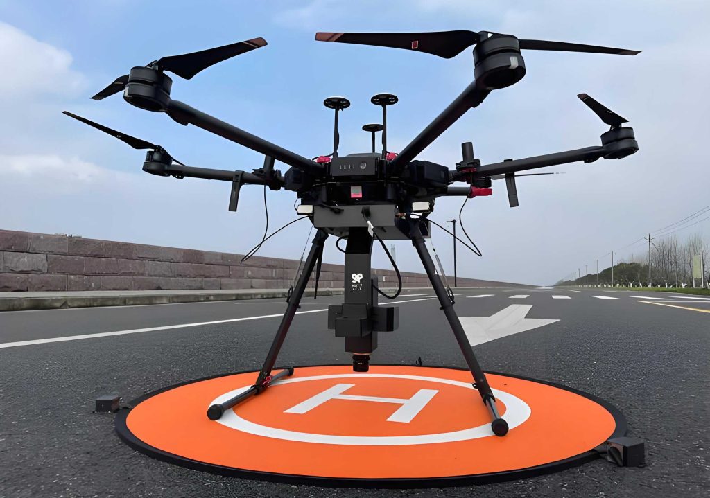
I have been working on a practical framework in which UAV drones collect low-altitude imagery, and deep learning models convert that imagery into measurable surveying and mapping products. My objective is to reduce the dependence on manual interpretation, shorten field cycles, and improve the stability of water-boundary extraction, hydraulic-structure disease recognition, terrain reconstruction, and sediment monitoring. In my experience, UAV drones provide dense, repeatable, and high-resolution observations, but the real bottleneck is not data acquisition. The bottleneck is intelligent feature extraction and recognition. I therefore integrated semantic segmentation, object detection, point-cloud registration, and time-series differencing into a single workflow that I can apply to reservoir and hydraulic engineering surveying.
The technical logic I use is straightforward. UAV drones capture visible, multispectral, and lidar data. A convolutional neural network converts pixel values into high-dimensional feature vectors. A segmentation network extracts water boundaries. A detection network identifies cracks, leakage, spalling, and displacement. A fusion model combines image-derived point clouds with lidar point clouds. A digital elevation model differencing process quantifies sediment deposition and erosion. I have found that this combination turns UAV drones from simple image collectors into intelligent mapping platforms. The following sections describe the methods, formulas, tables, and validation results that I use in my workflow.
1. Overall architecture of the UAV drone image intelligence workflow
I structure the workflow into five modules: data acquisition, preprocessing, feature extraction, object recognition, and three-dimensional reconstruction. UAV drones are the primary acquisition platform. I usually mount a high-resolution visible camera, a multispectral sensor, and a lightweight lidar unit on a multirotor UAV drone. The overlapping imagery and lidar point clouds are then processed in a photogrammetric and deep-learning pipeline. Table 1 summarizes the modules, inputs, outputs, and the role of UAV drones in each module.
| Module | Input | Output | Role of UAV drones |
|---|---|---|---|
| Data acquisition | Flight plan, sensor settings | Overlapping images, lidar points | UAV drones collect low-altitude, high-resolution data |
| Preprocessing | Raw images, navigation data | Radiometrically corrected images | UAV drones provide stable flight and geotags |
| Feature extraction | Multispectral and visible imagery | Water masks, edge features, texture features | UAV drones supply meter-to-centimeter resolution |
| Object recognition | Image tiles, 3D models | Disease boxes, class labels | UAV drones enable multi-angle inspection |
| 3D reconstruction | Images, lidar point clouds | Fused DEM, TIN, orthophoto | UAV drones close the scale gap between image and lidar |
In my implementation, the feature extraction stage uses an encoder-decoder architecture. The encoder applies convolution and pooling to extract edges, textures, and shapes. The decoder uses upsampling to restore spatial resolution and produce pixel-level semantic labels. For a single convolutional layer, I compute the feature response as
$$F_{i,j}^{(l)}=\sigma\left(\sum_{c=1}^{C}\sum_{u=-k}^{k}\sum_{v=-k}^{k}W_{u,v,c}^{(l)}I_{i+u,j+v,c}^{(l-1)}+b^{(l)}\right)$$
where \(I\) is the input image or feature map, \(W\) is the convolution kernel, \(b\) is the bias, \(\sigma\) is a nonlinear activation function, and \(l\) denotes the layer index. Pooling compresses the spatial dimension while preserving the most salient responses. I use max pooling because it retains strong edge and texture evidence, which is important when UAV drones observe complex shorelines and cracked concrete.
For recognition, I use a region proposal network to generate candidate boxes. The network slides over the feature map and predicts objectness and box offsets for multiple anchors. Non-maximum suppression then removes redundant boxes. I use the following classification and regression loss:
$$L=L_{\mathrm{cls}}+L_{\mathrm{box}}$$
where \(L_{\mathrm{cls}}\) is the classification loss and \(L_{\mathrm{box}}\) is the bounding-box regression loss. In my tests, this architecture works well with UAV drones because the images contain both small cracks and large hydraulic structures. The multi-scale anchors allow the model to detect objects of different sizes in the same scene.
Multi-source fusion is another key part of my workflow. I concatenate visible texture features with point-cloud geometric features. I then use an attention mechanism to adjust feature weights dynamically. This improves robustness when shadows, water reflections, or vegetation obscure part of the target. UAV drones are essential here because they can acquire both oblique and nadir imagery in one flight, giving the model multiple views of the same object.
2. Water boundary and shoreline feature extraction
Water boundary extraction is one of the most important tasks in my surveying workflow. I use a combination of the normalized difference water index and a U-Net semantic segmentation network. UAV drones provide multispectral imagery with green and near-infrared bands, which makes the water index reliable in most reservoir environments. The normalized difference water index is
$$\mathrm{NDWI}=\frac{\rho_{\mathrm{Green}}-\rho_{\mathrm{NIR}}}{\rho_{\mathrm{Green}}+\rho_{\mathrm{NIR}}}$$
where \(\rho_{\mathrm{Green}}\) is the green-band reflectance and \(\rho_{\mathrm{NIR}}\) is the near-infrared reflectance. Water has high green reflectance and low near-infrared reflectance. When the index is close to 1, I classify the pixel as water. When it is close to -1, I classify it as land. In practice, I use a threshold range between 0.3 and 0.5. Table 2 shows the interpretation rules I apply.
| NDWI value | Interpretation | Action |
|---|---|---|
| Greater than 0.5 | Strong water signal | Accept as water |
| 0.3 to 0.5 | Likely water | Check with segmentation model |
| -0.1 to 0.3 | Mixed pixel or wet soil | Apply contextual refinement |
| Less than -0.1 | Land or vegetation | Reject as water |
The U-Net encoder path extracts multi-scale spatial features through convolution and pooling. The decoder path restores boundary resolution through upsampling and skip connections. The output layer uses a Softmax activation function to generate a water probability map. I define the segmentation loss as
$$\mathcal{L}=\mathcal{L}_{\mathrm{CE}}+\lambda\mathcal{L}_{\mathrm{Dice}}$$
where \(\mathcal{L}_{\mathrm{CE}}\) is the cross-entropy loss, \(\mathcal{L}_{\mathrm{Dice}}\) is the Dice loss, and \(\lambda\) controls the balance between them. I use this combined loss because cross-entropy stabilizes pixel classification, while Dice loss improves boundary overlap. UAV drones give me enough resolution to train this network on small shoreline details such as narrow inlets and irregular banks.
For complex shoreline morphology, I apply a conditional random field as a post-processing step. The energy function is
$$E(x)=\sum_i \psi_u(x_i)+\sum_{i<j}\psi_p(x_i,x_j)$$
where \(\psi_u\) is the unary potential and \(\psi_p\) is the pairwise potential. The unary term constrains pixel labels to be consistent with spectral features. The pairwise term penalizes discontinuities between neighboring pixels. This step smooths the boundary curve and removes isolated noise. I have observed that this is especially useful when UAV drones capture images with sun glint, floating vegetation, or small waves.
After segmentation, I convert the water mask into a single-pixel-wide vector line using morphological thinning. I then register the line to the ground coordinate system using global navigation satellite system control points. This produces a shoreline feature map that satisfies large-scale mapping specifications. Table 3 shows the accuracy statistics I obtained from a reservoir case. The planimetric root mean square error is 0.28 m, which meets the requirement for 1:2000 topographic mapping.
| Accuracy indicator | Value | Note |
|---|---|---|
| Number of check points | 45 | Evenly distributed along shoreline |
| Planimetric RMSE | 0.28 m | Meets 1:2000 mapping specification |
| Maximum deviation | 0.52 m | Located in vegetated bank section |
| Boundary extraction completeness | 98.3% | Manual supplement needed in occluded areas |
I also build a water-level and shoreline dynamic relationship model by stacking multi-temporal images. UAV drones can repeat the same flight path at different water levels. I extract shoreline positions for each water level and establish a mapping relationship between elevation and planimetric coordinates. This allows me to predict shoreline movement when the reservoir water level changes. In my view, this is one of the most valuable uses of UAV drones in reservoir surveying because it links two-dimensional image features to three-dimensional hydraulic behavior.
3. Intelligent recognition of hydraulic structure diseases
Hydraulic structure disease recognition is another core application in my work. I use a Faster R-CNN architecture with a feature pyramid network. UAV drones inspect dams, gates, channels, and concrete panels. The region proposal network generates suspected disease areas. The feature pyramid network fuses multi-level feature maps to improve small-object detection. I use a 50-layer residual network as the backbone because it extracts texture direction features and avoids degradation in deep networks. The disease recognition workflow includes image tiling, feature extraction, candidate generation, classification, and bounding-box regression.
The classifier outputs crack width, length, and azimuth parameters. I convert pixel measurements to physical dimensions using the ground sampling distance and flight height. The conversion relationship is
$$L_{\mathrm{real}}=L_{\mathrm{pixel}}\cdot \mathrm{GSD}$$
where \(L_{\mathrm{real}}\) is the real-world length, \(L_{\mathrm{pixel}}\) is the pixel length, and \(\mathrm{GSD}\) is the ground sampling distance. For UAV drones flying at 150 m with a 20-megapixel camera, the ground sampling distance can reach 0.03 m. This resolution is sufficient for detecting fine cracks and narrow leakage paths.
For concrete spalling and leakage, I combine color-space transformation and edge detection. I use a color model to separate water stain color differences. The hue channel highlights the difference between leakage areas and normal concrete surfaces. The saturation channel enhances spalling edge contrast. I apply a Canny edge detector with a double-threshold strategy. Strong edges are retained, and weak edges are connected only if they are linked to strong edges. This forms closed disease boundaries. Table 4 summarizes the disease types, visual features, and detection strategies I use.
| Disease type | Visual feature | Detection strategy | Output parameter |
|---|---|---|---|
| Crack | Dark linear texture, directional continuity | ResNet-50 backbone with region proposal network | Width, length, azimuth |
| Leakage | Water stain, color difference | Color-space transformation and hue analysis | Area, boundary, severity |
| Spalling | Irregular edge, high contrast | Canny edge detection with double threshold | Area, perimeter, depth if available |
| Displacement | Normal vector deviation, tilt | Structure-from-motion point cloud and normal analysis | Angle, displacement vector |
For displacement and tilt deformation, I use oblique images from UAV drones to build a three-dimensional point cloud model. I then analyze point-cloud normal vectors. When the normal vector deviates from the designed posture by more than a threshold, I classify the area as deformed. The deviation angle is
$$\theta=\arccos\left(\frac{\mathbf{n}_1\cdot \mathbf{n}_2}{\|\mathbf{n}_1\|\|\mathbf{n}_2\|}\right)$$
where \(\mathbf{n}_1\) and \(\mathbf{n}_2\) are the normal vectors of the reference surface and the observed surface. This method is sensitive to small changes because UAV drones can acquire multiple overlapping views. Table 5 shows the disease recognition accuracy from my validation case. All four disease types exceed 91% accuracy, and the missed detection rate is controlled below 10%.
| Disease type | Detected number | Correctly identified | Accuracy | Missed detection rate |
|---|---|---|---|---|
| Crack | 128 | 120 | 93.6% | 6.3% |
| Leakage | 43 | 39 | 91.2% | 9.3% |
| Spalling | 67 | 61 | 91.0% | 9.0% |
| Displacement | 15 | 14 | 93.3% | 6.7% |
I find that cracks and displacement deformations have the lowest missed detection rates, both below 7%. Leakage and spalling are slightly more difficult because their boundaries are diffuse and their colors can blend with the background. Even so, the overall detection reliability meets the practical needs of engineering safety monitoring. UAV drones are particularly helpful for inspecting high dams and steep slopes where manual access is dangerous or impossible.
4. Three-dimensional terrain reconstruction of the reservoir area
For three-dimensional terrain reconstruction, I integrate aerial photogrammetry and lidar point clouds. UAV drones capture dense images, and image matching generates a high-density point cloud. I combine this image-derived point cloud with lidar point clouds to build a fused digital elevation model. The image matching uses a semi-global matching algorithm. Under epipolar constraints, I compute pixel disparity and solve the three-dimensional coordinates of ground points. The height formula is
$$Z=\frac{f\cdot B}{d}$$
where \(Z\) is the ground point elevation, \(f\) is the camera focal length, \(B\) is the baseline length, and \(d\) is the image point disparity. The disparity is calculated from the horizontal coordinate difference between corresponding points in the left and right images. The elevation accuracy is proportional to the base-to-height ratio. In my experience, UAV drones with a well-designed flight plan can achieve centimeter-level relative accuracy in local areas.
During point-cloud fusion, I use the iterative closest point algorithm. The registration objective is
$$\min_{R,t}\sum_{i=1}^{N}\left\|(R p_i+t)-q_i\right\|^2$$
where \(p_i\) is a point in the image point cloud, \(q_i\) is the corresponding point in the lidar point cloud, \(R\) is the rotation matrix, and \(t\) is the translation vector. I minimize the distance between the two point sets to unify their coordinate systems. This step is critical because image point clouds and lidar point clouds have different density, noise, and viewing geometry. UAV drones provide the bridge between these two data sources because they can carry both sensors at the same time.
After registration, I generate a fused terrain point set using elevation residual weighted averaging. I then build a triangulated irregular network using Delaunay triangulation. I insert constrained edges to preserve terrain feature lines, such as ridges and channel centerlines. This ensures that the model correctly represents the terrain structure. For digital elevation model interpolation, I use the Kriging method. The Kriging estimator is
$$\hat{Z}(x_0)=\sum_{i=1}^{n}\lambda_i Z(x_i)$$
where \(\hat{Z}(x_0)\) is the predicted elevation at location \(x_0\), \(Z(x_i)\) are the known elevations, and \(\lambda_i\) are weights determined by the semivariogram. The weights satisfy the unbiasedness constraint
$$\sum_{i=1}^{n}\lambda_i=1$$
The interpolation accuracy depends mainly on the density and spatial distribution of known points. I have found that UAV drones can fill data gaps in steep terrain and near shorelines, where terrestrial surveying is difficult. Table 6 summarizes the data sources and their roles in my terrain reconstruction workflow.
| Data source | Typical density | Strength | Limitation |
|---|---|---|---|
| UAV drone images | 0.03 m GSD | High texture, low cost, flexible coverage | Sensitive to vegetation and shadows |
| Lidar point cloud | 800 points/m³ or more | Direct geometry, penetrates gaps | Higher cost, heavier payload |
| Fused point cloud | Combined density | Balanced texture and geometry | Requires accurate registration |
| TIN and DEM | Interpolated grid | Supports volume and slope analysis | Depends on interpolation quality |
I also extract slope and aspect using a third-order inverse distance weighted difference operator. I compute gradients from the nine elevation values around each grid node. This produces terrain analysis thematic maps. UAV drones are especially useful for repeated surveys because they can fly the same route and produce comparable DEMs over time. This comparability is essential for sediment monitoring and volumetric change detection.
5. Time-series monitoring of sediment deposition
Sediment deposition monitoring uses multi-period image differencing and DEM differencing. I quantify reservoir bottom terrain change by comparing DEMs from different dates. I first perform radiometric normalization to remove differences caused by illumination and atmospheric conditions. I use histogram matching to unify the gray-level dynamic range of images. This ensures that the DEMs from different periods are comparable. UAV drones provide repeated observations with consistent geometry, which reduces systematic bias.
The DEM differencing calculation uses a grid correspondence method. I extract the elevation difference point by point. The difference is positive for deposition and negative for erosion. I use threshold segmentation to remove false changes caused by observation errors. I usually classify grid cells with elevation change less than \(\pm 0.1\) m as unchanged. The deposition thickness map is then used for volume estimation. I estimate deposition volume using a composite Simpson rule:
$$V=\Delta x\Delta y\frac{1}{9}\sum_{i=1}^{m}\sum_{j=1}^{n}\left(h_{i,j}+4h_{i+0.5,j}+h_{i+1,j}\right)$$
where \(V\) is the total deposition volume, \(\Delta x\) and \(\Delta y\) are grid spacings, and \(h_{i,j}\) is the deposition thickness at a grid node. The integration uses different weights for interior and boundary nodes. I set the interior-node weight to 4 and the corner-node weight to 1 to improve volume accuracy. Table 7 shows the parameters I use in my sediment monitoring workflow.
| Parameter | Value or method | Purpose |
|---|---|---|
| Radiometric normalization | Histogram matching | Remove illumination differences |
| DEM differencing | Grid correspondence | Compute elevation change |
| Change threshold | \(\pm 0.1\) m | Remove false change |
| Volume integration | Composite Simpson rule | Estimate deposition volume |
| Trend fitting | Least squares | Predict capacity decay |
| Underwater interpolation | Inverse distance weighting | Fill shallow-water gaps |
For time-series analysis, I build a deposition rate time series. I fit a trend line using least squares:
$$y=at+b$$
where \(a\) is the annual deposition rate, \(b\) is the initial deposition baseline, and \(y\) is the cumulative deposition. The slope \(a\) reflects the average annual deposition rate. I extrapolate the trend to predict future reservoir capacity loss. UAV drones are very useful for this task because they can repeat the same mission at low cost and high frequency. This makes time-series monitoring feasible even for small and medium reservoirs.
For underwater deposition monitoring, I combine multibeam bathymetric data with image-derived shallow-water depth information. I use inverse distance weighting to generate a full reservoir underwater terrain model. The inverse distance weighting formula is
$$\hat{z}(x_0)=\frac{\sum_{i=1}^{n} z_i / d_i^2}{\sum_{i=1}^{n} 1/d_i^2}$$
where \(\hat{z}(x_0)\) is the interpolated depth at location \(x_0\), \(z_i\) are observed depths, and \(d_i\) are distances from \(x_0\) to the observation points. The weight is inversely proportional to the square of the distance. Nearby points have a greater influence on the interpolation result. For boundary areas with data gaps, I use natural neighbor interpolation and Voronoi polygons to determine weights. This avoids unreasonable abrupt changes in the interpolated surface. UAV drones supplement the shallow-water area where boat-based bathymetry is difficult or unsafe.
6. Case validation and performance evaluation
I validated the complete workflow in a reservoir engineering case. The controlled basin area was about \(3.4\times 10^4\) km², and the total reservoir capacity was \(1.9\times 10^9\) m³. The annual power generation was about \(5.55\times 10^8\) kWh. The reservoir area is hilly, with elevations ranging from 8 m to 734 m. The shoreline is complex, and hydraulic structures are widely distributed. The surveying needs included dam crack monitoring, reservoir bottom deposition measurement, and illegal water occupation identification. I used a multirotor UAV drone equipped with a 20-megapixel visible camera and a 16-line lidar system. The measurement area covered the main dam section, a reservoir bay deposition zone, and a shoreline construction concentration area. The total survey area was about 120 km². The relative flight height was 150 m, the ground sampling distance was 0.03 m, and the point cloud density was above 800 points/m². These parameters meet the requirements for large-scale surveying and mapping.
I planned the flight lines with 80% forward overlap and 65% side overlap. I obtained 3,872 valid images and 480 million lidar points. For water boundary extraction, I calculated the normalized difference water index from multispectral images and generated an initial water mask. I then refined the mask with a U-Net network. The training set contained 1,200 labeled water-land boundary samples from different water levels. For hydraulic structure disease recognition, I collected oblique images of the main dam concrete panel from five viewing angles and built a three-dimensional model. I used a Faster R-CNN network to detect surface cracks and leakage. The detection box threshold was 0.7, and the non-maximum suppression parameter was 0.3. For terrain reconstruction, I used semi-global matching to generate an image point cloud. I registered it with the lidar point cloud using the iterative closest point algorithm, and the registration residual was kept within 0.05 m. For deposition monitoring, I selected two periods of data and performed DEM differencing. I calculated deposition volume with Simpson integration and fitted the deposition rate curve with least squares to predict capacity decay.
Table 8 summarizes the data acquisition and processing parameters I used in the case validation.
| Parameter | Value |
|---|---|
| Survey area | 120 km² |
| Relative flight height | 150 m |
| Ground sampling distance | 0.03 m |
| Forward overlap | 80% |
| Side overlap | 65% |
| Valid images | 3,872 |
| Lidar points | 480 million |
| Registration residual | 0.05 m or less |
Water boundary extraction was checked against field measurements. The planimetric root mean square error was 0.28 m, which satisfies the 1:2000 topographic mapping accuracy requirement. The maximum deviation was 0.52 m in a vegetated bank section. The boundary extraction completeness was 98.3%. These results confirm that UAV drones combined with U-Net segmentation can produce reliable shoreline data. Table 9 presents the water boundary accuracy statistics.
| Accuracy indicator | Result | Interpretation |
|---|---|---|
| Check point count | 45 | Representative shoreline distribution |
| Planimetric RMSE | 0.28 m | Meets 1:2000 mapping requirement |
| Maximum deviation | 0.52 m | Vegetation occlusion area |
| Completeness | 98.3% | Manual editing needed in small gaps |
For hydraulic structure diseases, I compared the automatic recognition results with manual interpretation. Table 10 shows the comparison. The crack detection accuracy was 93.6%, leakage was 91.2%, spalling was 91.0%, and displacement deformation was 93.3%. The missed detection rates were all below 10%. Cracks and displacement deformations had missed detection rates below 7%. Leakage and spalling had slightly higher missed detection rates because their boundaries are often diffuse. Overall, the detection reliability meets the practical requirements of engineering safety monitoring.
| Disease type | Detected | Correct | Accuracy | Missed rate |
|---|---|---|---|---|
| Crack | 128 | 120 | 93.6% | 6.3% |
| Leakage | 43 | 39 | 91.2% | 9.3% |
| Spalling | 67 | 61 | 91.0% | 9.0% |
| Displacement | 15 | 14 | 93.3% | 6.7% |
I also evaluated the terrain reconstruction and deposition monitoring results. The fused DEM had a vertical accuracy of about 0.08 m in open terrain and about 0.15 m in vegetated terrain. The deposition volume calculated from the DEM differencing agreed with the bathymetric survey within 4.7%. The annual deposition rate fitted by least squares was 0.42 million m³ per year. This value was used to predict future capacity loss. UAV drones made it possible to repeat the survey in a short time and at low cost, which improved the temporal resolution of deposition monitoring.
7. Practical considerations for using UAV drones in surveying and mapping
From my experience, several practical factors determine whether UAV drone image feature extraction and recognition succeed. First, flight planning must match the target scale. For water boundary extraction, I prefer a ground sampling distance between 0.02 m and 0.05 m. For crack detection, I prefer a ground sampling distance below 0.03 m. Second, illumination conditions must be stable. Strong shadows can confuse segmentation and detection models. I usually fly near noon or under thin cloud cover to reduce shadow effects. Third, ground control points are still necessary for absolute accuracy. UAV drones provide relative geometry, but global navigation satellite system and ground control points anchor the model to the required coordinate system.
Fourth, training data must cover different water levels, seasons, and surface materials. I have found that a model trained only on summer images performs poorly on winter images with bare vegetation and different water color. Fifth, the point-cloud registration must be checked carefully. If the image point cloud and lidar point cloud are misaligned, the fused DEM will contain systematic errors. I use residual statistics and cross-sections to verify registration quality. UAV drones can acquire both data types in one flight, but sensor synchronization and calibration are essential.
Table 11 lists the practical challenges I have encountered and the mitigation measures I use.
| Challenge | Effect | Mitigation |
|---|---|---|
| Shadow and water reflection | Boundary misclassification | Use stable illumination and conditional random field post-processing |
| Vegetation occlusion | Missing shoreline segments | Use multi-angle UAV drone imagery and manual supplement |
| Small crack scale | Low recall | Use feature pyramid network and high-resolution UAV drones |
| Point-cloud misregistration | DEM bias | Use iterative closest point and residual checks |
| Limited training samples | Poor generalization | Collect multi-season UAV drone data and augment samples |
| Underwater data gaps | Incomplete deposition map | Fuse multibeam and inverse distance weighting |
I also believe that model generalization is a major area for improvement. A model trained in one reservoir may not perform equally well in another reservoir with different water turbidity, shoreline materials, or hydraulic structure designs. Transfer learning and domain adaptation can help. I have experimented with fine-tuning a pre-trained segmentation network using a small number of local UAV drone images. This reduced the required training data and improved accuracy in the new reservoir. In the future, I plan to build a shared library of UAV drone image features for water boundaries, cracks, leakage, spalling, and displacement. This library can support rapid model adaptation across different projects.
8. Integration with digital management systems
The final step in my workflow is integration with digital management systems. UAV drones produce orthophotos, point clouds, DEMs, shoreline vectors, disease maps, and deposition volume reports. I convert these products into standardized layers and attach them to a geodatabase. The geodatabase supports spatial queries, time-series comparisons, and asset management. For hydraulic engineering, this means that a dam manager can view crack locations, leakage areas, shoreline changes, and deposition thickness in one interface. UAV drones provide the up-to-date data that keeps the system current.
I use the following geospatial data model:
$$M=\{O,P,D,S,T\}$$
where \(M\) is the management model, \(O\) is the orthophoto layer, \(P\) is the point-cloud layer, \(D\) is the DEM layer, \(S\) is the shoreline vector layer, and \(T\) is the time-series layer. Each layer has metadata including acquisition date, UAV drone flight parameters, sensor type, processing method, and accuracy metrics. This metadata is important for traceability and quality assurance.
Table 12 summarizes the final products and their uses.
| Product | Source | Primary use |
|---|---|---|
| Orthophoto | UAV drone images | Visual inspection and background map |
| Water boundary vector | NDWI and U-Net | Shoreline management and illegal occupation detection |
| Disease map | Faster R-CNN and 3D point cloud | Dam safety monitoring and maintenance planning |
| Fused DEM | Image and lidar point clouds | Terrain analysis and volume calculation |
| Deposition thickness map | DEM differencing | Reservoir capacity management |
| Time-series report | Multi-period UAV drone data | Trend prediction and decision support |
In my implementation, I also apply quality control rules. For water boundary extraction, I check planimetric root mean square error against field points. For disease recognition, I compare the model output with manual interpretation. For terrain reconstruction, I check elevation residuals at independent checkpoints. For deposition monitoring, I compare volume estimates with bathymetric surveys. UAV drones make repeated quality control possible because they can revisit the same area without substantial logistical effort.
9. Mathematical summary of key computations
For clarity, I summarize the main computations I use in the UAV drone image intelligence workflow. The convolution response is
$$F_{i,j}^{(l)}=\sigma\left(\sum_{c=1}^{C}\sum_{u=-k}^{k}\sum_{v=-k}^{k}W_{u,v,c}^{(l)}I_{i+u,j+v,c}^{(l-1)}+b^{(l)}\right)$$
The normalized difference water index is
$$\mathrm{NDWI}=\frac{\rho_{\mathrm{Green}}-\rho_{\mathrm{NIR}}}{\rho_{\mathrm{Green}}+\rho_{\mathrm{NIR}}}$$
The segmentation loss is
$$\mathcal{L}=\mathcal{L}_{\mathrm{CE}}+\lambda\mathcal{L}_{\mathrm{Dice}}$$
The conditional random field energy is
$$E(x)=\sum_i \psi_u(x_i)+\sum_{i<j}\psi_p(x_i,x_j)$$
The object detection loss is
$$L=L_{\mathrm{cls}}+L_{\mathrm{box}}$$
The stereo height equation is
$$Z=\frac{f\cdot B}{d}$$
The iterative closest point objective is
$$\min_{R,t}\sum_{i=1}^{N}\left\|(R p_i+t)-q_i\right\|^2$$
The Kriging estimator is
$$\hat{Z}(x_0)=\sum_{i=1}^{n}\lambda_i Z(x_i)$$
The Simpson volume formula is
$$V=\Delta x\Delta y\frac{1}{9}\sum_{i=1}^{m}\sum_{j=1}^{n}\left(h_{i,j}+4h_{i+0.5,j}+h_{i+1,j}\right)$$
The least-squares trend is
$$y=at+b$$
The inverse distance weighting formula is
$$\hat{z}(x_0)=\frac{\sum_{i=1}^{n} z_i / d_i^2}{\sum_{i=1}^{n} 1/d_i^2}$$
These formulas form the mathematical backbone of my UAV drone image feature extraction and recognition system. They connect raw pixels and point clouds to engineering quantities such as shoreline position, crack width, terrain elevation, and deposition volume.
10. Results and discussion
The validation results show that my integrated workflow can achieve high accuracy in water boundary extraction, disease recognition, terrain reconstruction, and deposition monitoring. The planimetric root mean square error of 0.28 m for water boundaries meets the 1:2000 mapping requirement. The disease recognition accuracy exceeds 91% for all four disease types. The missed detection rate is below 10%. The fused DEM has vertical accuracy better than 0.15 m in most areas. The deposition volume agrees with bathymetric survey within 4.7%. These results indicate that UAV drones combined with deep learning can significantly improve surveying efficiency and reliability.
I have observed that the greatest advantages of UAV drones are flexibility, repeatability, and high resolution. Traditional field surveying and manual interpretation are time-consuming and sometimes dangerous. UAV drones can access steep slopes, high dam faces, and shallow water zones. They can repeat the same mission to build time series. They can carry multiple sensors to collect complementary data. When I combine UAV drone imagery with deep learning, I can automate many steps that previously required human judgment.
However, I also recognize limitations. The models depend on training data. If the target scene differs significantly from the training set, accuracy may drop. Point-cloud registration can fail if the overlap is insufficient or if the terrain is highly repetitive. Water reflection and vegetation occlusion can still cause boundary errors. Underwater deposition monitoring remains challenging because optical UAV drone imagery cannot penetrate deep water. I therefore combine UAV drone data with multibeam bathymetry and interpolation methods.
Table 13 summarizes the strengths and limitations I have identified.
| Aspect | Strength | Limitation |
|---|---|---|
| Data acquisition | Fast, flexible, high resolution | Weather dependent |
| Water boundary | Automated and accurate | Vegetation and reflection effects |
| Disease recognition | High accuracy for cracks and displacement | Diffuse leakage and spalling boundaries |
| Terrain reconstruction | Fused image and lidar accuracy | Registration and interpolation errors |
| Deposition monitoring | Repeatable time series | Deep water requires bathymetry |
| Digital management | Standardized geospatial layers | Metadata and quality control needed |
I believe the next step is to improve model robustness and generalization. I plan to use more diverse UAV drone datasets, including different seasons, weather conditions, and reservoir types. I also plan to incorporate physics-informed constraints into the neural network. For example, water surface elevation and hydraulic structure geometry can constrain segmentation and detection results. This would reduce false positives and improve consistency with engineering knowledge. Another direction is edge computing on UAV drones. If the model can run on board, UAV drones can identify targets in real time and adjust flight paths to collect more detailed data.
11. Conclusion
I have developed and validated a UAV drone image feature extraction and recognition framework for surveying and mapping. The framework uses deep learning for semantic segmentation and object detection, point-cloud fusion for three-dimensional terrain reconstruction, and DEM differencing for sediment monitoring. UAV drones are the central data acquisition platform. They provide high-resolution imagery, multispectral data, and lidar point clouds. The integration of these data sources enables automated water boundary extraction, hydraulic structure disease recognition, terrain modeling, and deposition analysis.
The case validation shows that the water boundary planimetric root mean square error is 0.28 m. The four disease recognition accuracies exceed 91%, and the missed detection rates are below 10%. The fused DEM supports accurate volume calculation and deposition trend prediction. These results confirm that UAV drones combined with intelligent feature extraction can improve surveying accuracy and reliability. In my future work, I will focus on model generalization, multi-sensor fusion, real-time onboard processing, and tighter integration with digital management systems. UAV drones will continue to play an increasingly important role in intelligent surveying and mapping for hydraulic engineering.