
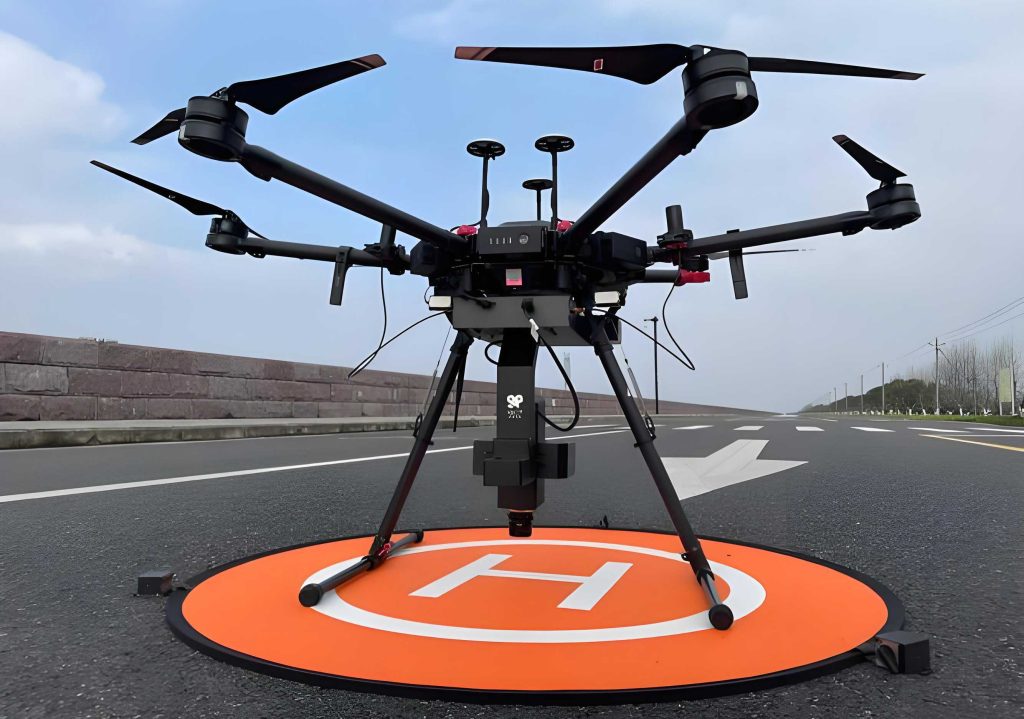
Object detection from the perspective of UAV drones is not merely a scaled-down version of generic visual recognition. In my work, I treat it as a coupled problem of weak early texture, inconsistent cross-scale spatial support, and unreliable high-order context aggregation. UAV drones frequently operate at high altitude, where vehicles, pedestrians, cyclists, and other targets occupy only a few pixels. The background is dense and cluttered, scale variation is extreme, and small objects lack discriminative texture. These factors jointly degrade the reliability of node representations before any attention, matching, or fusion mechanism can act. I therefore propose LHM-DEIM, a detector built on a DEIM-DFINE-style baseline, which introduces three coordinated components: a Laplacian-of-Gaussian initial feature extraction module, a hypergraph hybrid encoding neck, and a mutual guided fusion module. The design follows a simple principle: improve the reliability of shallow nodes, align them into a common spatial domain, aggregate high-order relations on that domain, and feed the resulting context back to detection scales.
In my formulation, the input image is first transformed into a multi-scale feature set. Let the backbone stages produce feature maps \(\mathbf{P}_2,\mathbf{P}_3,\mathbf{P}_4,\mathbf{P}_5\). For UAV drones, \(\mathbf{P}_2\) contains the strongest spatial detail, while \(\mathbf{P}_5\) contains the strongest semantic abstraction. The difficulty is that these maps live on different grids, different receptive fields, and different noise levels. A detector that simply concatenates or adds them cannot guarantee that a node at one scale is comparable with a node at another scale. I address this by making the spatial support explicit and by using hypergraph computation to model group-wise relations among similar nodes.
1. Problem Setting and Baseline
I use a DEIM-DFINE architecture as the baseline because it provides a strong real-time detection transformer with improved matching and fine-grained distribution refinement. However, the baseline still struggles when UAV drones capture highly complex scenes. The baseline can be summarized as a mapping from an image \(\mathbf{I}\) to a set of predictions \(\hat{\mathbf{Y}}\):
$$
\hat{\mathbf{Y}} = \mathcal{D}\left(\mathcal{E}\left(\mathcal{B}(\mathbf{I})\right)\right)
$$
where \(\mathcal{B}\) is the backbone, \(\mathcal{E}\) is the hybrid encoder neck, and \(\mathcal{D}\) is the decoder. In my improved model, the mapping becomes:
$$
\hat{\mathbf{Y}} = \mathcal{D}\left(\mathcal{F}_{\mathrm{MGF}}\left(\mathcal{H}_{\mathrm{Hyper}}\left(\mathcal{A}_{\mathrm{SSA}}\left(\mathcal{S}_{\mathrm{LoG}}(\mathbf{I})\right)\right)\right)\right)
$$
Here, \(\mathcal{S}_{\mathrm{LoG}}\) is the LoGStem module, \(\mathcal{A}_{\mathrm{SSA}}\) is the spatial scale alignment mechanism, \(\mathcal{H}_{\mathrm{Hyper}}\) is the hypergraph computation module, and \(\mathcal{F}_{\mathrm{MGF}}\) is the mutual guided fusion module. The rest of this article explains each component, provides the mathematical formulation, and reports extensive experiments on VisDrone2019 and UAVDT. Throughout, I emphasize why each design choice matters for UAV drones rather than treating the modules as independent add-ons.
2. Method
The overall architecture of LHM-DEIM has three parts: a backbone with a LoGStem front end, a hybrid encoder neck named H-HEN, and a decoder. The information flow is deliberately closed-loop. Shallow detail is enhanced first, then aligned, then aggregated, and finally returned to the detection scales. This is important because UAV drones often produce images in which the same object can appear as a tiny cluster of pixels in one region and as a larger structure in another. Without a shared spatial reference, relation modeling can connect a target node to a background node simply because their raw feature distances are small after inconsistent downsampling.
2.1 LoGStem: Laplacian-of-Gaussian Initial Feature Extraction
In my design, the first stage of the backbone is replaced by LoGStem. The motivation is direct: for UAV drones, weak edges and low contrast are common. A standard stem may suppress high-frequency spatial information before the network has a chance to encode it. LoGStem combines a differentiable Laplacian-of-Gaussian edge prior, a Gaussian residual branch, and a multi-scale structure fusion path. The module improves node discriminability at the source, which later helps distance-based hypergraph construction avoid connecting targets with background clutter.
Let \(\mathbf{F}_0\) be the initial feature after a \(7\times7\) convolution. The LoG filter branch computes:
$$
\mathbf{F}_{\mathrm{LoG}} = \phi\left(\mathrm{BN}\left(\mathbf{F}_0\right)\right) + \phi\left(\mathrm{BN}\left(\mathbf{F}_0 \ast \mathbf{K}_{\mathrm{LoG}}\right)\right)
$$
where \(\ast\) denotes depthwise convolution, \(\mathbf{K}_{\mathrm{LoG}}\) is the LoG kernel, \(\mathrm{BN}(\cdot)\) is batch normalization, and \(\phi(\cdot)\) is the SiLU activation. This residual form preserves the original response while injecting an edge-enhanced response. For UAV drones, this is beneficial because small vehicles and pedestrians often have weak but consistent boundaries. The LoG prior makes those boundaries more separable before the first aggressive downsampling step.
After edge enhancement, high-frequency noise may remain. I therefore apply a Gaussian residual branch on an intermediate downsampled feature \(\mathbf{F}_D\):
$$
\mathbf{F}_{G} = \phi\left(\mathrm{BN}\left(\mathbf{F}_D\right)\right) + \phi\left(\mathrm{BN}\left(\mathbf{F}_D \ast \mathbf{K}_{G}\right)\right)
$$
Here \(\mathbf{K}_{G}\) is a channel-adaptive Gaussian kernel. Unlike hard pooling or strided convolution, this branch performs weighted spatial aggregation and retains high-frequency details through the residual connection. The combination is important for UAV drones because over-smoothing can erase the very evidence that distinguishes a small target from a textured roof or road marking.
The multi-scale structure fusion path, which I call DRFD, decouples high-frequency enhancement and low-frequency aggregation. Two parallel branches are used:
$$
\mathbf{F}_{c} = \phi\left(\mathrm{BN}\left(\mathrm{Conv}_{3\times3}\left(\mathbf{F}, s=2\right)\right)\right)
$$
$$
\mathbf{F}_{m} = \phi\left(\mathrm{BN}\left(\mathrm{MaxPool}_{3\times3}\left(\mathbf{F}, s=2\right)\right)\right)
$$
Then the two branches are concatenated and compressed:
$$
\mathbf{F}_{\mathrm{stem}} = \mathrm{Conv}_{1\times1}\left(\left[\mathbf{F}_{c}, \mathbf{F}_{m}\right]\right)
$$
The output \(\mathbf{F}_{\mathrm{stem}}\) has resolution \(H/4 \times W/4\) and serves as the input to the subsequent backbone stages. Table 1 summarizes the role of each LoGStem submodule for UAV drones.
| Submodule | Operation | Primary benefit for UAV drones |
|---|---|---|
| LoG filter | Depthwise LoG convolution with residual | Enhances weak edges and fine contours of small objects |
| Gaussian residual | Channel-adaptive Gaussian smoothing with residual | Suppresses sensor noise while preserving high-frequency detail |
| DRFD | Parallel convolution and max-pooling branches | Balances texture preservation and low-frequency context |
| Stem output | \(1\times1\) channel compression | Produces a compact representation for later alignment and hypergraph modeling |
The effect of LoGStem is not limited to local enhancement. Because hypergraph construction depends on Euclidean distances between node features, unreliable shallow features can cause false edges. If a small target has a weak response and a background patch has a similar weak response, a distance threshold may group them together. LoGStem reduces this risk by making target boundaries and textures more distinguishable at the earliest stage. In my experiments, this translates into consistent gains in average precision and small-object average precision.
2.2 H-HEN: Hypergraph Hybrid Encoding Neck
Traditional feature pyramid networks and path aggregation networks transmit information across scales, but they do not explicitly define a common grid on which nodes from different scales should be compared. For UAV drones, this omission is costly. A node from \(\mathbf{P}_2\) and a node from \(\mathbf{P}_5\) may correspond to the same physical location, yet their feature vectors are computed on different resolutions and receptive fields. I therefore design H-HEN to first align all scales to a common spatial support and then perform hypergraph-based context aggregation on that support.
2.2.1 Spatial Scale Alignment
I use \(\mathbf{P}_4\) as the reference scale. The choice is deliberate: \(\mathbf{P}_4\) is an intermediate scale that retains useful localization detail while carrying sufficient semantic information. The features \(\mathbf{P}_2,\mathbf{P}_3,\mathbf{P}_4,\mathbf{P}_5\) are mapped to the \(\mathbf{P}_4\) grid through downsampling, identity mapping, or upsampling:
$$
\mathbf{P}_{2\rightarrow4} = D_2\left(\mathbf{P}_2\right)
$$
$$
\mathbf{P}_{3\rightarrow4} = D_1\left(\mathrm{Conv}_{1\times1}\left(\mathbf{P}_3\right)\right)
$$
$$
\mathbf{P}_{4\rightarrow4} = \mathrm{Conv}_{1\times1}\left(\mathbf{P}_4\right)
$$
$$
\mathbf{P}_{5\rightarrow4} = U\left(\mathrm{Trans}\left(\mathrm{Conv}_{1\times1}\left(\mathbf{P}_5\right)\right)\right)
$$
Here \(D_2(\cdot)\) and \(D_1(\cdot)\) denote two and one downsampling operations, \(U(\cdot)\) denotes upsampling, and \(\mathrm{Trans}(\cdot)\) is a transformer block applied to the highest-level feature to capture global dependencies. After this step, all four branches have the same spatial resolution as \(\mathbf{P}_4\). I concatenate them along the channel dimension and compress the result with a \(1\times1\) convolution:
$$
\mathbf{F}_{\mathrm{enc}} = \mathrm{Conv}_{1\times1}\left(\left[\mathbf{P}_{2\rightarrow4}, \mathbf{P}_{3\rightarrow4}, \mathbf{P}_{4\rightarrow4}, \mathbf{P}_{5\rightarrow4}\right]\right)
$$
This alignment has a precise role in my architecture. It creates a shared index set so that every spatial position carries local texture, cross-scale semantics, and global context. Without this step, hypergraph nodes would be compared across incompatible grids. With this step, the distance threshold \(\epsilon\) constrains a meaningful neighborhood in a common representation space. Table 2 summarizes the SSA branches and their contributions.
| Branch | Operation | Role in the aligned representation |
|---|---|---|
| \(\mathbf{P}_2 \rightarrow \mathbf{P}_4\) | Two downsampling operations | Injects high-resolution detail for small targets |
| \(\mathbf{P}_3 \rightarrow \mathbf{P}_4\) | One downsampling operation and \(1\times1\) convolution | Adds mid-level structure and local context |
| \(\mathbf{P}_4 \rightarrow \mathbf{P}_4\) | Identity grid and \(1\times1\) convolution | Provides the reference representation |
| \(\mathbf{P}_5 \rightarrow \mathbf{P}_4\) | Transformer, \(1\times1\) convolution, and upsampling | Supplies global semantic dependencies |
I note that downsampling \(\mathbf{P}_2\) is not a lossless operation. Some high-frequency detail is compressed. However, the design still provides a favorable trade-off because it avoids adding an independent \(\mathbf{P}_2\) detection head, which would increase computation and memory. For UAV drones with limited edge resources, this is an important practical consideration. The aligned feature \(\mathbf{F}_{\mathrm{enc}}\) becomes the input to the hypergraph computation module.
2.2.2 Distance-Based Hypergraph Construction and Context Enhancement
After obtaining \(\mathbf{F}_{\mathrm{enc}}\), I flatten the spatial dimensions and treat each position as a node. Let \(\mathbf{x}_i\) be the feature vector of node \(i\). The Euclidean distance between nodes \(i\) and \(j\) is:
$$
D_{ij} = \left\| \mathbf{x}_i – \mathbf{x}_j \right\|_2, \quad i,j = 1,2,\ldots,N
$$
The binary hypergraph incidence matrix is defined by a threshold \(\epsilon\):
$$
\mathbf{H}_{ij} =
\begin{cases}
1, & D_{ij} \lt \epsilon \\
0, & D_{ij} \ge \epsilon
\end{cases}
$$
Each node defines an \(\epsilon\)-ball hyperedge that contains all nodes within distance \(\epsilon\) in the feature space. This construction preserves symmetry and allows one hyperedge to cover multiple related nodes. It can represent group relations that pairwise graph edges cannot easily express. For UAV drones, this is useful because a small object may be partially occluded or may appear as several weak responses. A hyperedge can aggregate evidence from multiple neighboring nodes that belong to the same object or the same local context.
The threshold \(\epsilon\) is not an arbitrary constant. It controls the locality of high-order information propagation. If \(\epsilon\) is too small, a hyperedge contains too few nodes, and context from complementary parts of the same target is lost. If \(\epsilon\) is too large, background nodes such as road, roof, and vegetation are absorbed into the same hyperedge, which dilutes the target representation. In my sensitivity analysis on VisDrone2019, \(\epsilon = 128\) gives the best balance. I report this in detail later.
The HyperCompute module performs two-stage message passing. First, node features \(\mathbf{X}\) are linearly transformed:
$$
\mathbf{X}’ = \mathbf{X}\mathbf{W}, \quad \mathbf{W} \in \mathbb{R}^{C \times C}
$$
Then the incidence matrix is normalized:
$$
\mathbf{P} = \mathrm{Normalize}\left(\mathbf{H}\right), \quad
\mathbf{P}_{ij} = \frac{\mathbf{H}_{ij}}{\sum_{k=1}^{N}\mathbf{H}_{ik}}
$$
The first aggregation produces hyperedge representations:
$$
\mathbf{E} = \mathrm{Agg}\left(\mathbf{H}^{\top}, \mathbf{X}’\right)
$$
The second aggregation produces updated node representations:
$$
\hat{\mathbf{X}} = \mathrm{Agg}\left(\mathbf{H}, \mathbf{E}\right)
$$
Finally, a residual connection and normalization are applied:
$$
\mathbf{F}_{\mathrm{hyp}} = \phi\left(\mathrm{BN}\left(\hat{\mathbf{X}}\right)\right) + \mathbf{X}
$$
The first message-passing stage preserves the commonality of similar nodes and suppresses accidental responses from isolated noisy nodes. The second stage gives each node both its original local representation and the context of its hyperedge. The residual connection ensures that if the neighborhood relation is unreliable, the original feature can still be transmitted. This prevents over-smoothing of small objects, which is a serious concern for UAV drones because excessive smoothing can erase the few pixels that distinguish a target from the background.
Table 3 summarizes the H-HEN components and their effect on detection.
| Component | Function | Effect on UAV drone detection |
|---|---|---|
| Spatial scale alignment | Maps \(\mathbf{P}_2\) to \(\mathbf{P}_5\) to the \(\mathbf{P}_4\) grid | Creates a common spatial support for cross-scale comparison |
| Distance-based hypergraph | Builds \(\epsilon\)-ball hyperedges from feature distances | Models group-wise relations among similar nodes |
| HyperCompute | Two-stage message passing with normalization | Aggregates high-order context while preserving local detail |
| Residual connection | Adds the original node feature | Prevents over-smoothing of small targets |
In my interpretation, H-HEN addresses a specific failure mode of UAV drones: the same object may be represented by multiple weak nodes, while the background may contain many nodes with similar weak responses. Pairwise attention may propagate noise from background to target. Hypergraph aggregation with a controlled radius can instead require group consensus, which improves robustness. This is why I combine spatial scale alignment with hypergraph construction rather than using either alone.
2.3 MutualGuideFusion
The hypergraph module produces context-enriched features on the aligned \(\mathbf{P}_4\) grid. However, detection still requires features at multiple scales. If the context remains only in the encoder, the decoder may not benefit fully. I therefore design MutualGuideFusion to feed the high-order context back to the detection scales. The module takes two feature maps, typically \(\mathbf{P}_4\) and \(\mathbf{P}_5\), and performs bidirectional information exchange with channel recalibration.
First, the two inputs are aligned in channel dimension using \(1\times1\) convolutions:
$$
\mathbf{P}’_i = \mathrm{Conv}_{1\times1}\left(\mathbf{P}_i\right)
$$
Then squeeze-and-excitation attention is applied to recalibrate channel responses:
$$
\mathbf{P}^{\mathrm{att}}_i = \mathrm{SEAttention}\left(\mathbf{P}’_i\right)
$$
The bidirectional fusion is formulated as:
$$
\mathbf{P}^{\mathrm{fused}}_i = \mathbf{P}^{\mathrm{att}}_i \odot \mathbf{P}_i
$$
Finally, a \(1\times1\) convolution adjusts the output dimension:
$$
\mathbf{F}_{\mathrm{out}} = \mathrm{Conv}_{1\times1}\left(\mathbf{P}^{\mathrm{fused}}\right)
$$
Here \(\odot\) denotes element-wise multiplication after broadcast to the appropriate spatial size. The SE attention mechanism computes global average pooling, two fully connected layers, and a sigmoid gate. It adaptively emphasizes target-related channels and suppresses background channels. In my model, the high-level context from \(\mathbf{P}_5\) helps suppress background responses in \(\mathbf{P}_4\), while the fine-grained structure in \(\mathbf{P}_4\) constrains the over-abstraction of \(\mathbf{P}_5\). This mutual guidance is especially valuable for UAV drones because small targets often share colors and textures with the background.
Table 4 presents the effect of each MutualGuideFusion operation.
| Operation | Formula | Purpose |
|---|---|---|
| Channel projection | \(\mathbf{P}’_i = \mathrm{Conv}_{1\times1}(\mathbf{P}_i)\) | Matches channel dimensions before fusion |
| SE recalibration | \(\mathbf{P}^{\mathrm{att}}_i = \mathrm{SEAttention}(\mathbf{P}’_i)\) | Re-weights channels by global importance |
| Bidirectional fusion | \(\mathbf{P}^{\mathrm{fused}}_i = \mathbf{P}^{\mathrm{att}}_i \odot \mathbf{P}_i\) | Exchanges complementary information across scales |
| Output projection | \(\mathbf{F}_{\mathrm{out}} = \mathrm{Conv}_{1\times1}(\mathbf{P}^{\mathrm{fused}})\) | Produces decoder-ready features |
I emphasize that the three main modules are not independent. LoGStem improves the local identifiability of nodes. SSA places nodes from different scales into a common spatial domain. HyperCompute aggregates high-order relations on that domain. MutualGuideFusion returns the aggregated context to the detection scales. The pipeline forms a closed loop from low-level detail to high-level context and back. In my ablation studies, removing any one module reduces performance, and combining all three yields the best results.
3. Experiments and Analysis
3.1 Dataset and Implementation Details
I evaluate LHM-DEIM on VisDrone2019 and UAVDT. VisDrone2019 contains 10,209 static images, with 6,471 training images, 548 validation images, and 3,190 test images. It covers diverse urban and suburban scenes captured by UAV drones. The dataset is challenging because small objects account for a large proportion of instances, and occlusion is frequent. UAVDT contains 40,735 high-resolution images, with 24,143 for training and 16,592 for validation. It focuses on cars, buses, and trucks under different altitudes, viewpoints, weather conditions, and illumination conditions. I use UAVDT to test generalization.
All experiments are conducted with Torch 2.3.0, CUDA 12.1, Python 3.10.16, and Torchvision 0.18.0 on an RTX 4090 GPU with 24 GB memory. Input images are resized to \(640\times640\). I use batch size 4, an initial learning rate of \(10^{-4}\), and FP32 precision without automatic mixed precision. The reason is that HyperCompute builds discrete hyperedges from Euclidean distances and a fixed threshold \(\epsilon\). Mixed precision can introduce rounding differences near the threshold, which may change hyperedge connectivity. To ensure fair comparison, all experiments use the same FP32 setting.
3.2 Ablation Study
I first evaluate the contribution of LoGStem, H-HEN, and MutualGuideFusion. Table 5 reports the results on VisDrone2019. The metrics include \(\mathrm{AP}\), \(\mathrm{AP}_{0.5}\), \(\mathrm{AP}_s\), and parameter count.
| Setting | LoGStem | H-HEN | MutualGuideFusion | \(\mathrm{AP}_{0.5}\)/% | \(\mathrm{AP}\)/% | \(\mathrm{AP}_s\)/% | Params/\(10^6\) |
|---|---|---|---|---|---|---|---|
| Baseline | — | — | — | 34.3 | 19.3 | 12.3 | 3.73 |
| 1 | ✓ | — | — | 35.1 | 19.6 | 12.9 | 3.76 |
| 2 | — | ✓ | — | 36.2 | 20.1 | 13.5 | 3.83 |
| 3 | — | — | ✓ | 35.3 | 19.8 | 12.9 | 3.74 |
| 4 | ✓ | ✓ | — | 37.3 | 20.5 | 13.7 | 3.86 |
| 5 | ✓ | — | ✓ | 35.7 | 19.7 | 13.1 | 3.78 |
| 6 | — | ✓ | ✓ | 36.7 | 20.9 | 13.9 | 3.85 |
| 7 | ✓ | ✓ | ✓ | 38.2 | 21.6 | 14.8 | 3.89 |
The results show that each module improves the baseline. LoGStem alone raises \(\mathrm{AP}_{0.5}\) by 0.8 percentage points and \(\mathrm{AP}\) by 0.3 percentage points. This confirms that early texture enhancement benefits UAV drones. H-HEN alone raises \(\mathrm{AP}_{0.5}\) by 1.9 percentage points and \(\mathrm{AP}\) by 0.8 percentage points, with a small increase in parameters. MutualGuideFusion alone raises \(\mathrm{AP}_{0.5}\) by 1.0 percentage point with only a marginal parameter increase. The full model improves \(\mathrm{AP}_{0.5}\) from 34.3% to 38.2%, \(\mathrm{AP}\) from 19.3% to 21.6%, and \(\mathrm{AP}_s\) from 12.3% to 14.8%, while parameters increase by about 4.3%. This is a favorable accuracy-efficiency trade-off for UAV drones.
I also perform a detailed ablation of H-HEN. Table 6 shows the effect of SSA and HyperCompute separately and together.
| Model | \(\mathrm{AP}_{0.5}\)/% | \(\mathrm{AP}\)/% | \(\mathrm{AP}_s\)/% | Params/\(10^6\) |
|---|---|---|---|---|
| Baseline | 34.3 | 19.3 | 12.3 | 3.73 |
| SSA only | 35.2 | 19.6 | 12.9 | 3.76 |
| HyperCompute only | 35.4 | 19.9 | 13.1 | 3.81 |
| Full H-HEN | 36.2 | 20.1 | 13.5 | 3.83 |
SSA alone improves \(\mathrm{AP}_{0.5}\) by 0.9 percentage points, showing that spatial alignment reduces scale-induced feature distortion. HyperCompute alone improves \(\mathrm{AP}_s\) to 13.1%, showing that high-order relations help small objects. When combined, the full H-HEN achieves 36.2% \(\mathrm{AP}_{0.5}\) and 13.5% \(\mathrm{AP}_s\), with only a 2.7% parameter increase over the baseline. This demonstrates that the two mechanisms are complementary.
3.3 Sensitivity to the Hypergraph Threshold
The threshold \(\epsilon\) controls hyperedge radius. I test five values: 64, 96, 128, 160, and 192. Table 7 reports the results on VisDrone2019.
| \(\epsilon\) | \(\mathrm{AP}_{0.5}\)/% | \(\mathrm{AP}\)/% | \(\mathrm{AP}_s\)/% |
|---|---|---|---|
| 64 | 36.4 | 19.9 | 13.2 |
| 96 | 37.8 | 20.9 | 13.9 |
| 128 | 38.2 | 21.6 | 14.8 |
| 160 | 37.6 | 20.7 | 13.4 |
| 192 | 36.6 | 19.8 | 13.3 |
Performance first increases and then decreases as \(\epsilon\) grows. A small \(\epsilon\) limits the context coverage of each hyperedge, while a large \(\epsilon\) includes weakly related or background nodes and introduces relation noise. The best result is obtained at \(\epsilon = 128\), with 38.2% \(\mathrm{AP}_{0.5}\), 21.6% \(\mathrm{AP}\), and 14.8% \(\mathrm{AP}_s\). The decline in \(\mathrm{AP}_s\) is especially noticeable when \(\epsilon\) becomes too large, which suggests that very small objects are more sensitive to background noise entering the hyperedge. This supports my design choice of using a moderate radius for UAV drones.
3.4 Comparison with State-of-the-Art Detectors
I compare LHM-DEIM with representative detectors, including Faster R-CNN, Cascade R-CNN, DINO, YOLOv8, YOLOv11, YOLOv12, FBRT-YOLO-S, YOLO26, RT-DETR variants, and two DEIM-based methods. Table 8 reports the results on VisDrone2019.
| Model | \(\mathrm{AP}\)/% | \(\mathrm{AP}_{0.5}\)/% | \(\mathrm{AP}_s\)/% | \(\mathrm{AP}_m\)/% | \(\mathrm{AP}_l\)/% | Params/\(10^6\) | GFLOPs | FPS |
|---|---|---|---|---|---|---|---|---|
| Faster R-CNN-R50 | 19.4 | 32.9 | 9.5 | 30.9 | 42.9 | 41.39 | 208 | — |
| Cascade R-CNN-R50 | 19.7 | 32.6 | 9.9 | 30.9 | 40.6 | 69.29 | 236 | — |
| DINO | 25.3 | 44.5 | 15.1 | 37.1 | 50.3 | 47.56 | 274 | — |
| YOLOv8n | 19.2 | 32.3 | 9.9 | 28.8 | 33.9 | 3.1 | 8.1 | 86 |
| YOLOv8s | 21.4 | 37.6 | 12.3 | 30.3 | 36.2 | 11.13 | 28.5 | 51 |
| YOLOv11n | 19.3 | 31.3 | 9.7 | 27.9 | 33.6 | 2.59 | 6.3 | 94 |
| YOLOv11s | 21.6 | 38.4 | 12.6 | 31.2 | 36.2 | 9.42 | 21.3 | 56 |
| YOLOv12n | 19.2 | 31.4 | 9.6 | 27.7 | 34.6 | 2.56 | 6.3 | — |
| YOLOv12s | 21.5 | 38.6 | 12.4 | 30.8 | 35.8 | 9.23 | 21.2 | — |
| FBRT-YOLO-S | 20.3 | 36.9 | 11.8 | 29.6 | 35.3 | 2.9 | 22.9 | — |
| YOLO26s | 18.8 | 35.6 | 10.8 | 29.2 | 34.9 | 9.47 | 20.5 | — |
| RTDETR-R18 | 21.3 | 38.9 | 13.9 | 28.5 | 38.3 | 20 | 60 | — |
| RTDETRV2-R18 | 22.2 | 40.1 | 13.7 | 32.1 | 40.1 | 20 | 60 | — |
| HMF-DEIM | 23.5 | 40.5 | 14.8 | 34.6 | 48.9 | 11.87 | 34.1 | — |
| SCA-DEIM-N | 19.5 | 33.9 | 11.3 | 32.7 | 39.6 | 3.87 | 7.06 | — |
| LHM-DEIM | 21.6 | 38.2 | 14.8 | 31.3 | 36.9 | 3.89 | 16.4 | 54 |
LHM-DEIM achieves 21.6% \(\mathrm{AP}\), matching YOLOv11s and outperforming RTDETR-R18 and YOLOv12s. Its \(\mathrm{AP}_s\) of 14.8% is particularly strong, surpassing RTDETRV2-R18 by 1.1 percentage points and matching HMF-DEIM. The parameter count is only 3.89M and GFLOPs are 16.4, far below DINO and RT-DETR variants. This shows that LHM-DEIM offers a better balance between accuracy and efficiency for UAV drones.
I also evaluate embedded inference on a Jetson Orin Nano 4 GB platform with TensorRT 8.6.2, FP16 precision, \(640\times640\) input, and batch size 1. LHM-DEIM reaches 54 FPS, which is comparable to YOLOv8s and YOLOv11s while providing higher small-object precision. Compared with SCA-DEIM-N, LHM-DEIM improves \(\mathrm{AP}\), \(\mathrm{AP}_{0.5}\), and \(\mathrm{AP}_s\) by 2.1, 4.3, and 3.5 percentage points, respectively, at a similar parameter scale. Compared with HMF-DEIM, it has 1.9 percentage points lower overall \(\mathrm{AP}\) but the same \(\mathrm{AP}_s\), while reducing parameters by about 67.2% and computation by about 51.9%. This is a strong result for resource-constrained UAV drones.
3.5 Visualization and Generalization
I visualize detection results and heatmaps for challenging scenes, including daytime streets, dense parking lots, and nighttime roads. The baseline often produces missed detections in shadowed areas and distant small-object regions. LHM-DEIM reduces these misses and produces more concentrated heatmap responses. In dense parking lots, the baseline spreads activation over background textures, while LHM-DEIM focuses on target centers. In nighttime scenes, LHM-DEIM maintains recall under difficult illumination.
I also examine three challenging conditions: extremely small targets, heavy occlusion, and strong fog. In extremely small target scenes, the baseline has dispersed responses over vegetation and non-target regions, whereas LHM-DEIM concentrates on roads, vehicles, and target-dense areas. In occlusion scenes, LHM-DEIM forms more continuous responses over densely packed targets and maintains attention on partially occluded objects. In foggy scenes, the baseline generates many low-confidence proposals, while LHM-DEIM is more conservative and focuses on regions with remaining discriminative features. However, fog remains a difficult condition with missed detections, which indicates a direction for future improvement.
Table 9 reports the generalization results on UAVDT.
| Model | \(\mathrm{AP}\)/% | \(\mathrm{AP}_{0.5}\)/% | \(\mathrm{AP}_s\)/% | \(\mathrm{AP}_m\)/% | \(\mathrm{AP}_l\)/% | Params/\(10^6\) |
|---|---|---|---|---|---|---|
| Baseline | 19.1 | 32.1 | 14.8 | 28.1 | 30.3 | 3.73 |
| LHM-DEIM | 20.9 | 34.9 | 15.3 | 31.0 | 31.4 | 3.89 |
LHM-DEIM improves \(\mathrm{AP}\) by 1.8 percentage points, \(\mathrm{AP}_{0.5}\) by 2.8 percentage points, and \(\mathrm{AP}_s\) by 0.5 percentage points on UAVDT. The parameter increase is only 0.16M. This confirms that the improvements generalize to another UAV drone dataset with different scenes, altitudes, and weather conditions.
4. Discussion
The experiments support three conclusions. First, early texture enhancement is important for UAV drones because small targets can lose discriminative information before the first few downsampling stages. Second, cross-scale spatial alignment is necessary before relation modeling. Without it, hypergraph nodes from different scales are not directly comparable. Third, high-order context must be returned to the detection scales; otherwise it remains isolated in the encoder. LHM-DEIM combines these principles in a single architecture.
I also note limitations. HyperCompute uses a fixed distance threshold \(\epsilon\). Although \(\epsilon = 128\) works well on VisDrone2019, image degradation, target density, and feature distribution may vary across datasets. A fixed threshold can make neighborhoods too sparse or too dense. The choice of \(\mathbf{P}_4\) as the alignment reference is also static. For extremely small or extremely large targets, another scale or a dynamic mixture of scales may be better. LoG enhancement helps weak edges, but under strong noise or severe blur, a more reliable degradation-aware mechanism is needed. Spatial scale alignment may also face challenges under extreme occlusion or very small object localization.
Future work can address these limitations in several ways. I plan to learn adaptive thresholds from local feature density, prediction uncertainty, or task loss. I also plan to dynamically select or fuse alignment references such as \(\mathbf{P}_3\), \(\mathbf{P}_4\), and \(\mathbf{P}_5\) based on target scale distribution. Another direction is to jointly model LoG edge enhancement and image quality assessment so that high-frequency enhancement adapts to noise and blur. Finally, quantization, pruning, and distillation can further reduce computation for edge deployment on UAV drones while preserving small-object accuracy.
5. Conclusion
I have presented LHM-DEIM, a UAV-oriented object detection algorithm built on a DEIM-DFINE baseline. The method introduces LoGStem for Laplacian-of-Gaussian initial feature extraction, H-HEN for spatial scale alignment and hypergraph-based high-order context aggregation, and MutualGuideFusion for bidirectional multi-scale feature integration. On VisDrone2019, LHM-DEIM improves \(\mathrm{AP}_{0.5}\) from 34.3% to 38.2%, \(\mathrm{AP}\) from 19.3% to 21.6%, and \(\mathrm{AP}_s\) from 12.3% to 14.8%, with only a 4.3% parameter increase. On UAVDT, it improves \(\mathrm{AP}\) by 1.8 percentage points and \(\mathrm{AP}_{0.5}\) by 2.8 percentage points. These results show that LHM-DEIM is robust, practical, and well suited to the difficult conditions faced by UAV drones. The design also provides a foundation for future adaptive thresholding, dynamic scale alignment, and edge-efficient deployment in low-altitude remote sensing applications.