
Unmanned aerial vehicles possess a well-recognized capability for rapid deployment and reliable Line‑of‑Sight (LoS) connectivity. In the context of future mobile edge computing and emergency communication networks, unmanned aerial vehicles can be used as mobile base stations or flying computation servers to serve scattered ground terminals with on‑demand coverage. Nevertheless, several practical obstacles prevent the direct adoption of trajectory planning algorithms on physical platforms: high deployment cost, safety risks in cluttered environments, and mismatch between simulated and real channel conditions. Therefore, building a high‑fidelity simulation and digital‑twin environment for unmanned aerial vehicles is a necessary step toward efficient algorithm development and safe implementation.
In this work, I develop a simulation platform based on the Prometheus open‑source framework, integrate a real‑world 3D scene modelling pipeline using oblique photography and monocular vision, and propose a joint computational strategy and trajectory planning optimization algorithm for a UAV‑assisted MEC system. The effectiveness and versatility of the platform and the proposed algorithm are evaluated through systematic experiments. Detailed descriptions of the methodology, algorithm derivation, implementation steps, and quantitative comparison results are provided in the rest of this article.
| Symbol | Meaning |
|---|---|
| $q_n$ | UAV horizontal coordinate at segment $n$ |
| $z_n$ | UAV altitude at segment $n$ |
| $u_m$ | Horizontal coordinate of ground terminal $m$ |
| $W_m = (D_m, T_m, R_m)$ | Computation task request of terminal $m$ |
| $a_m$ | Task offloading ratio of terminal $m$ |
| $c_m$ | UAV caching ratio of task $W_m$ |
| $r_{mn}$ | Data rate between terminal $m$ and UAV at segment $n$ |
1. Introduction
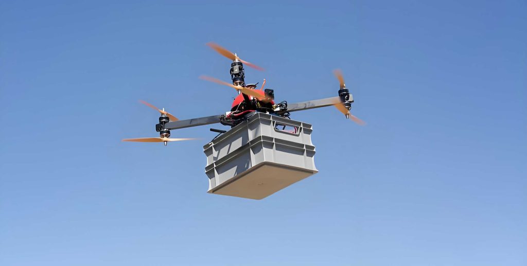
The emergence of bandwidth‑hungry and latency‑sensitive applications has imposed unprecedented pressure on terrestrial communication infrastructure. Fixed base stations are characterized by long deployment cycles and limited flexibility, especially in remote or disaster‑affected areas. Unmanned aerial vehicles offer a promising alternative because of their three‑dimensional mobility, fast deployment, and high probability of LoS propagation.
Despite the benefits, several critical challenges remain:
- Energy limitation: the on‑board battery capacity of unmanned aerial vehicles strictly limits their service time. Both propulsion and communication/computation energy must be minimized.
- Safe navigation: in realistic urban or indoor environments, the trajectory of unmanned aerial vehicles must be planned to avoid collisions with static and dynamic obstacles.
- Simulation-to-real gap: theoretical algorithms validated on idealized simulation platforms often fail in real flight tests because the virtual environment does not faithfully represent the actual terrain and obstacle layout.
- Coupled optimization: in a typical MEC system, the trajectory of unmanned aerial vehicles affects both the channel quality and the propulsion energy consumption, while the computation offloading and caching decisions affect the task delays and energy. These dimensions must be optimized jointly.
This article addresses these issues through a systematic investigation. The main contributions are as follows:
- I build a Prometheus-based simulation platform for unmanned aerial vehicles and extend it with a UAV-assisted communication trajectory planning module and a digital‑twin data exchange interface.
- I propose a 3D scene modelling method combining oblique photography and monocular vision for unmanned aerial vehicles, which enables high‑fidelity virtual environments.
- I formulate a joint optimization problem for task offloading, UAV caching, and three-dimensional trajectory, and solve it using iterative convex optimization techniques.
2. Simulation Platform for UAV-Assisted Communication
2.1 Platform Selection
Existing simulation environments for unmanned aerial vehicles can be categorized into three groups: game-engine-based platforms, network-level simulators, and robot-operation-system-based simulators. A comparison of these platforms is presented in the following table.
| Category | Advantages | Limitations | Suitable Scenarios |
|---|---|---|---|
| Game-engine-based (e.g., AirSim, Flightmare) | High visual fidelity; rich sensor data | Heavy resource consumption; poor network modelling; difficult ROS integration | Computer vision; semantic SLAM |
| Network-level (e.g., NS-3, OMNeT++) | Detailed protocol/channel modelling | Lack of UAV dynamics and 3D motion modelling | Throughput, delay, packet loss analysis |
| PX4-ROS based | Accurate dynamics; complete flight control | Complex setup; scattered modules | Sensor simulation; flight controller testing |
| Prometheus | Integrated modules for control, planning, vision, simulation | Some modules require further optimization | Secondary development; custom algorithm verification |
As can be seen, Prometheus provides an appropriate balance between physical fidelity, modularity, and flexibility. Therefore, I choose it as the core experimental platform.
2.2 System Architecture
The Prometheus software system is based on Ubuntu, ROS, Gazebo, and PX4. Its layered architecture comprises a simulation layer, a functional module layer, and a user interface layer. All layers communicate through ROS topics, services, and actions.
The bottom layer, Gazebo, simulates rigid-body dynamics, sensor measurements, and physical interactions. The PX4 Software-In-The-Loop (SITL) module runs the real flight-control stack. Above this, Prometheus provides state estimation, perception, planning, and control modules. I extended the original trajectory planning module by replacing the manual-target mode with a preset-target mode that continuously serves multiple ground terminals.
The core nodes and their functions are summarized below.
| Node | Function |
|---|---|
gazebo |
Runs the physics engine and sensor simulation |
uav1/mavros |
Bridge between ROS and PX4 flight stack |
joy_node |
Remote-control command processing |
uav_control_main_1 |
State machine management and command forwarding |
ego_planner |
Gradient-based B-spline local trajectory optimization |
2.3 Numerical Model of UAV Propulsion Energy
For a rotary-wing UAV, the propulsion energy consumption at trajectory segment $n$ can be modelled as
$$
E_n^{\mathrm{prop}} = \Delta_t \left( d_0 \rho s G v_n^q + P_0 \left(1 + \frac{3 (v_n^q)^2}{U_{\mathrm{tip}}^2}\right) + P_1 \sqrt{\sqrt{1 + \frac{(v_n^q)^4}{4 v_0^4}} – \frac{(v_n^q)^2}{2 v_0^2}} + \frac{1}{2} P_2 (v_n^z)^2 \right)
$$
where
- $d_0$ is the fuselage drag ratio,
- $\rho$ is the air density,
- $s$ is the rotor solidity,
- $G$ is the rotor disc area,
- $U_{\mathrm{tip}}$ is the rotor blade tip speed,
- $v_0$ is the mean rotor induced velocity in hover,
- $P_0$, $P_1$, and $P_2$ are blade profile power, induced power, and climb/descent power constants, respectively.
2.4 Digital Twin Module
To bridge the gap between simulation and physical execution, I design a digital-twin module based on a client-server architecture. The Prometheus simulation platform acts as the TCP socket server, and the physical UAV acts as the client. The workflow is as follows:
- The trajectory optimization module generates an optimal waypoint sequence.
- The virtual UAV in Gazebo receives position commands via ROS topics.
- When the virtual UAV reaches a waypoint, the server sends the coordinates to the physical UAV via TCP in JSON format.
- The physical UAV executes the waypoint flight task.
- The physical UAV state is fed back to the simulation platform to close the loop.
Experimental results show that the trajectory of the physical UAV closely matches that of the virtual UAV, confirming the effectiveness of the digital-twin mechanism.
3. 3D Scene Modelling for Trajectory Planning
3.1 Motivation
Most existing simulation platforms rely on manually designed virtual scenes. However, such scenes cannot accurately represent real terrain relief and obstacle distributions. This mismatch leads to significant performance degradation when transferring algorithms trained in simulation to physical flights. To solve this problem, I develop a three-dimensional scene reconstruction approach that integrates oblique photography and monocular visual perception.
3.2 Oblique Photography
Oblique photography captures both vertical and tilted perspectives using multi-lens camera systems on unmanned aerial vehicles. The collected images are processed through a standard photogrammetric pipeline, including data pre-processing, aerial triangulation, dense image matching, mesh generation, and texture mapping.
Aerial triangulation based on the collinearity equation is fundamental for determining the camera pose and the 3D coordinates of tie points:
$$
x – x_0 = -f \frac{a_1 (X – X_S) + b_1 (Y – Y_S) + c_1 (Z – Z_S)}{a_3 (X – X_S) + b_3 (Y – Y_S) + c_3 (Z – Z_S)}
$$
$$
y – y_0 = -f \frac{a_2 (X – X_S) + b_2 (Y – Y_S) + c_2 (Z – Z_S)}{a_3 (X – X_S) + b_3 (Y – Y_S) + c_3 (Z – Z_S)}
$$
where $(x,y)$ denotes the image point, $(x_0,y_0)$ is the principal point, $f$ is the focal length, $(X,Y,Z)$ is the object point, $(X_S,Y_S,Z_S)$ is the camera centre, and $a_i, b_i, c_i$ are the rotation matrix elements.
3.3 Coordinate Transformation for Monocular Vision
For monocular visual perception, I establish the mapping between the pixel coordinate system, image coordinate system, camera coordinate system, and world coordinate system. The pixel-to-image transformation is
$$
u = \frac{x}{dx} + u_0, \quad v = \frac{y}{dy} + v_0
$$
where $dx, dy$ are the physical dimensions of a single pixel, and $(u_0, v_0)$ is the principal point coordinate.
The image-to-camera transformation follows from the pinhole model:
$$
x = f \frac{X_c}{Z_c}, \quad y = f \frac{Y_c}{Z_c}
$$
The camera-to-world transformation is
$$
\begin{bmatrix} X_c \\ Y_c \\ Z_c \\ 1 \end{bmatrix}
= \begin{bmatrix} R & T \\ 0^T & 1 \end{bmatrix}
\begin{bmatrix} X_w \\ Y_w \\ Z_w \\ 1 \end{bmatrix}
$$
where $R$ is the rotation matrix and $T$ is the translation vector.
The PnP (Perspective-n-Point) algorithm is then applied to estimate the target pose and dimensions. The projection equation is given by
$$
s \begin{bmatrix} u \\ v \\ 1 \end{bmatrix}
= \mathbf{K} \begin{bmatrix} R & t \end{bmatrix}
\begin{bmatrix} X \\ Y \\ Z \\ 1 \end{bmatrix}
$$
where $s$ is the scale factor and $\mathbf{K}$ is the camera intrinsic matrix. To enhance robustness, I employ a fusion strategy based on PnP iterative solving with a triangle-similarity fallback. The system also adopts a distance-confidence-weighted averaging mechanism to further improve the stability of the estimated target dimensions.
3.4 Modelling Pipeline
The complete 3D scene modelling workflow consists of three stages.
| Stage | Processing | Output |
|---|---|---|
| 1. Initial modelling | Images imported into Context Capture; automatic aerial triangulation; dense matching; mesh and texture generation | DAE 3D model with real textures |
| 2. Local refinement | Monocular vision-based target size/distance estimation; PnP fusion solving; geometry correction | Precise local geometry |
| 3. Gazebo integration | Collision model generation; SDF description; world file creation | Gazebo-simulated real environment |
Quantitative evaluation of the reconstructed scene is conducted using the Context Capture quality reports. Key indicators include the connection point reprojection error, the image position uncertainty, and the ground resolution. The results show that for a laboratory environment reconstructed from 66 images:
- Calibration rate: 100%
- Median reprojection error: 0.6 pixels
- RMS reprojection error: 0.78 pixels
- Mean X-direction positional uncertainty: 0.00289
- Mean Y-direction positional uncertainty: 0.00235
- Mean Z-direction positional uncertainty: 0.00308
These values indicate high matching accuracy and satisfy the fidelity requirements for trajectory planning simulations.
3.5 Platform Integration Test
After generating the SDF model of the reconstructed scene, I integrate it into the Gazebo environment and launch the Prometheus platform for joint testing. The results show that the UAV can take off, hover, and navigate within the custom real-world model. When an obstacle is present, the onboard depth perception module detects it and the planner generates a feasible avoidance path in real time. This confirms the applicability of the reconstructed environment for complex trajectory planning experiments.
4. Joint Trajectory Planning and Computation Optimization in MEC Systems
4.1 System Model
I consider a UAV-assisted MEC system in which a single rotary-wing UAV serves $M$ ground terminals. The UAV carries an edge server and moves in three-dimensional space. The mission period is divided into $N$ time slots, each with duration $\Delta_t$. The horizontal coordinate and altitude of the UAV at segment $n$ are denoted by $q_n = (x_n, y_n)$ and $z_n$, respectively. The ground terminal $m$ is located at $u_m = (x_m, y_m)$ and generates a computation task $W_m = (D_m, T_m, R_m)$.
The channel gain between the UAV and terminal $m$ at segment $n$ depends on the LoS/NLoS condition and is written as
$$
g_{mn} = \frac{\xi_L \eta_L}{l_{mn}} \, p_{mn}^{\mathrm{LoS}} + \frac{\xi_N \eta_N}{l_{mn}} \, p_{mn}^{\mathrm{NLoS}}
$$
where $l_{mn} = \|q_n – u_m\|^2 + z_n^2$ is the squared Euclidean distance, $p_{mn}^{\mathrm{LoS}}$ is the LoS probability, $\xi_L$, $\xi_N$ are the path-loss coefficients, and $\eta_L$, $\eta_N$ are the corresponding exponents.
The achievable data rate at segment $n$ is given by the Shannon formula:
$$
r_{mn} = B \log_2 \left(1 + \frac{\rho_m g_{mn}}{\sigma^2}\right)
$$
4.2 Timing and Energy Model
Let $a_m \in [0,1]$ denote the offloading ratio and $c_m \in [0,1]$ the UAV caching ratio. The average transmission rate for terminal $m$ is
$$
\bar{r}_m = \frac{1}{N} \sum_{n=1}^{N} r_{mn}
$$
The computation latency of terminal $m$ is given by
$$
L_m = a_m \left( \frac{D_m}{\bar{r}_m} + \frac{R_m}{f_m^u} \right) + \frac{(1-a_m)R_m}{f_m^g}
$$
For the caching ratio $c_m$, the adjusted latency is
$$
L_m^a = L_m + (1-c_m) a_m \frac{R_m}{f_m^u}
$$
Similarly, the computation energy of terminal $m$ is expressed as
$$
E_m^a = E_m^u + E_m^g
$$
where
$$
E_m^u = a_m \kappa R_m \left( f_m^u \right)^2
$$
and
$$
E_m^g = (1-a_m) \times \frac{\kappa R_m \left( f_m^g \right)^2}{\rho_m D_m / \bar{r}_m}
$$
4.3 Optimization Problem
The overall service energy is the sum of the UAV propulsion energy and the computational energy:
$$
E_{\mathrm{all}} = \sum_{n=1}^{N} E_n^{\mathrm{prop}} + \sum_{m=1}^{M} E_m^a
$$
The optimization problem is then formulated as
$$
P: \min_{Q,Z,A,C} \; E_{\mathrm{all}}
$$
subject to
$$
\|q_{n+1} – q_n\|^2 \le \Delta_q^{\max}
$$
$$
|z_{n+1} – z_n| \le \Delta_z^{\max}, \quad z_{\min} \le z_n \le z_{\max}
$$
$$
\sum_{m=1}^{M} c_m D_m \le C_c
$$
$$
\sum_{m=1}^{M} a_m f_m^u \le C_u
$$
$$
L_m^a \le T_m
$$
$$
J_c = 0
$$
where the last constraint guarantees collision-free trajectory by enforcing zero collision cost.
4.4 Proposed Solution
Problem $P$ is non-convex due to the coupling between trajectory variables and computational variables, as well as the non-convex communication constraints. To address this, I decompose the original problem into three sub-problems and solve them iteratively.
Sub-problem 1: Computation energy minimization. With $Q$ and $Z$ fixed, the offloading ratios $A$ and caching ratios $C$ are optimized. The offloading sub-problem is
$$
P_1: \min_A \sum_{m=1}^{M} E_m^a
$$
subject to the computation capacity constraint. The caching sub-problem is
$$
P_2: \min_C \sum_{m=1}^{M} c_m D_m
$$
subject to the cache capacity constraint.
Sub-problem 2: Horizontal trajectory optimization. With $Z$, $A$, and $C$ fixed, the horizontal trajectory $Q$ is optimized to minimize propulsion energy while satisfying the communication rate constraint. I introduce slack variables to convexify the non-convex constraints. The rate constraint is replaced by
$$
\sum_{n=1}^{N} r_{mn} \ge N \bar{r}_m^{\min} \zeta
$$
where $\zeta \in [0,1]$ is a slack variable representing the minimum quality of service level.
Sub-problem 3: Vertical trajectory optimization. With $Q$, $A$, and $C$ fixed, the altitude sequence $Z$ is optimized by minimizing the total squared altitude variation:
$$
P_6: \min_Z \sum_{n=1}^{N} (z_{n+1} – z_n)^2
$$
subject to the altitude bound constraints and the communication rate constraint.
Once a new trajectory is obtained, the collision cost $J_c$ is checked. If a collision is detected, additional constraints are imposed to push the trajectory away from the obstacle. The algorithm iterates until convergence is achieved. The algorithm is summarized in the following pseudo-code.
| Algorithm 1: Joint UAV offloading, caching, and trajectory optimization | |
|---|---|
| 1: | Initialize trajectory $Q^0$, $Z^0$; iteration index $n=0$; set $A^0$, $C^0$ |
| 2: | repeat |
| 3: | Compute average data rates $r_{mn}$ based on current trajectory |
| 4: | Solve $P_1$ using IPOPT to obtain offloading ratios $A^{e}$ |
| 5: | Solve $P_2$ using IPOPT to obtain caching ratios $C^{e}$ |
| 6: | Solve $P_4$ using IPOPT to obtain horizontal trajectory $Q^{e}$ |
| 7: | Solve $P_6$ using IPOPT to obtain altitude $Z^{e}$ |
| 8: | Check collision constraint $J_c = 0$; when violated, add constraints and re-optimize |
| 9: | Update $Q = Q^e$, $Z = Z^e$; $n = n+1$ |
| 10: | until the decrease of $E_{\mathrm{all}}$ is smaller than the convergence threshold |
| 11: | Publish the optimized trajectory to the flight controller |
4.5 Experimental Results
To evaluate the proposed algorithm, I integrate it into the Prometheus platform with a Gazebo environment containing obstacles such as buildings, trees, and pedestrians. The main simulation parameters are listed in the table below.
| Parameter | Value |
|---|---|
| Bandwidth $B$ | 2.0 GHz |
| Terminal transmit power $\rho_m$ | 5 mW |
| Noise density $N_0$ | −169 dBm/Hz |
| LoS path-loss coefficient $\xi_L$ | 1.995 |
| NLoS path-loss coefficient $\xi_N$ | 1.259 |
| Hover induced power $P_1$ | 6.72 W |
| Blade profile power $P_0$ | 0.67 W |
| Climb/descent power $P_2$ | 11.46 W |
| Maximum speed | 1.0 m/s |
| Maximum acceleration | 1.0 m/s² |
| Obstacle inflation distance | 0.3 m |
| Takeoff height | 1.5 m |
| Planning horizon | 10 m |
| Map size | 150 m × 150 m × 3 m |
4.5.1 Data Rate Improvement
I compare the proposed optimized scheme with a baseline scheme that follows a straight-line trajectory and a reference scheme that offloads all tasks to the UAV. In terms of the average data rate of each ground terminal, the optimized scheme achieves a notable improvement over the initial scheme. This is because the optimized trajectory tends to pass closer to the ground terminals, thereby improving the effective channel gain. The performance gap becomes more significant when $M=6$ than when $M=5$, indicating that the trajectory optimization is more beneficial in dense deployments.
4.5.2 Latency Reduction
For the cumulative task transmission delay, the proposed scheme achieves a reduction of approximately $39.14\%$ compared with the initial scheme and $56.23\%$ compared with the full-offloading reference scheme when $M=5$. When $M=6$, the reductions are $43.6\%$ and $61.4\%$, respectively. These improvements stem from the joint optimization of offloading/caching decisions and trajectory adjustments.
4.5.3 Energy Savings
For the cumulative computation energy, the proposed scheme reduces energy consumption by about $52.02\%$ compared with the initial scheme and $76.93\%$ compared with the full-offloading reference scheme when $M=5$. For $M=6$, the corresponding reductions are $48.9\%$ and $76.5\%$. When considering the total service energy, the proposed scheme achieves a reduction of $3.18\%$ and $9.77\%$ for $M=5$, and $3.69\%$ and $11.77\%$ for $M=6$, respectively.
These results validate the effectiveness of the joint optimization approach. The platform also enables visual observation of real-time UAV states, such as position, altitude, velocity, and obstacle distance, during the optimization-enabled flight.
5. Conclusion
In this work, I have designed a Prometheus-based simulation platform for the development and validation of trajectory planning algorithms for unmanned aerial vehicles in assisted communication scenarios. The platform supports high-fidelity physical simulation, customized trajectory planning, and digital-twin data exchange between simulated and physical unmanned aerial vehicles. Additionally, I have proposed a three-dimensional scene modelling method that integrates oblique photography and monocular vision, thereby improving the consistency between the simulated environment and the real world. Finally, I have formulated and solved a joint computation-caching-trajectory optimization problem for a UAV-assisted MEC system. Simulation results confirm that the proposed scheme enhances data rates, reduces task latency, and lowers system energy consumption while ensuring collision-free flight.
In future work, I plan to extend the proposed approach to multi-UAV cooperative systems, incorporate dynamic obstacle avoidance and uncertain channel conditions, and further integrate deep reinforcement learning with convex optimization to improve the adaptability and scalability of trajectory planning algorithms for unmanned aerial vehicles.