
In the rapid development of urban low-altitude airspace, unmanned aerial vehicles (UAVs) have been widely deployed in logistics delivery, infrastructure inspection, environmental monitoring, and emergency rescue operations. While the autonomous obstacle avoidance capability of these unmanned aerial vehicles has advanced significantly, the question of system failure remains a critical safety concern. The unpredictable nature of urban environments—ranging from glass curtain walls to rapidly moving ground vehicles—presents challenges that even the most sophisticated sensing and decision-making algorithms cannot fully overcome. When the autonomous obstacle avoidance system of unmanned aerial vehicles ceases to function correctly, the consequences can be catastrophic, leading to collisions, uncontrollable descent, and potential ground casualties.
My research is motivated by the urgent need to develop systematic emergency strategies that activate precisely when autonomous obstacle avoidance fails. The key insight of this work is that a human-in-the-loop intervention mechanism, built upon a robust understanding of operator reaction times and a well-designed multi-strategy obstacle avoidance framework, can significantly enhance the safety of unmanned aerial vehicles in degraded operational conditions. Throughout this thesis, I employ a combination of theoretical modeling, controlled experiments, and simulation-based validation to explore how unmanned aerial vehicles can maintain safe flight even when their primary autonomous systems break down.
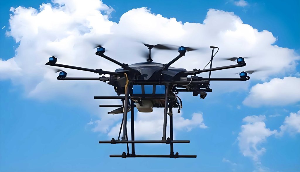
1. Introduction and Research Context
The adoption of unmanned aerial vehicles in civilian domains has grown exponentially over the past decade. In modern logistics systems, for instance, these unmanned aerial vehicles perform last-mile deliveries in dense urban areas where ground transportation faces significant congestion. In the energy sector, unmanned aerial vehicles inspect power lines and offshore platforms, reducing human exposure to hazardous environments. The common thread across these applications is the reliance on autonomous flight capabilities, particularly the ability to sense and avoid obstacles in real time. However, my literature review reveals that while substantial research has been devoted to improving the nominal performance of obstacle avoidance algorithms, relatively little attention has been paid to the failure modes of these systems and the associated emergency protocols.
The existing body of research on obstacle avoidance for unmanned aerial vehicles can be broadly classified into two categories: global path planning methods and local collision avoidance methods. The former includes algorithms such as A*, Dijkstra’s algorithm, Rapidly-exploring Random Trees (RRT), and Probabilistic Roadmaps (PRM), which rely on pre-existing or partially known environmental information. The latter, including Artificial Potential Fields (APF) and Dynamic Window Approach (DWA), processes real-time sensor data to generate immediate avoidance maneuvers. Through my analysis, I find that both categories exhibit vulnerabilities in unstructured urban environments. The global planners suffer from computational latency and environmental map inaccuracies, whereas the local methods frequently fail when confronted with unexpected obstacles or degraded sensor performance.
| Algorithm Category | Representative Methods | Core Philosophy | Limitations in Failure Scenarios |
|---|---|---|---|
| Global Path Planning | A*, Dijkstra, RRT, PRM | Search for a collision-free path from start to goal in a known environment | High computational overhead, poor adaptability to dynamic changes |
| Local Collision Avoidance | APF, DWA, Learning-based | Real-time velocity/heading adjustment based on local sensor data | Susceptible to sensor noise, limited perception range |
| Hybrid Approaches | D* Lite, Anytime D* | Re-planning in dynamic environments based on incremental search | Complex implementation, still requires reliable sensor inputs |
Another dimension of my literature review focuses on understanding the behavioral aspects of unmanned aerial vehicles operators. Specifically, I examined the research on human reaction time—a critical parameter that determines the effectiveness of manual intervention in emergency scenarios. Studies from the automotive domain, such as those by Lechner and others, demonstrate that human reactions are not purely instantaneous physiological responses but are deeply influenced by cognitive load, experience, and environmental complexity. The research by Tang and Xia on driver reaction times provided an analogous foundation for my work on unmanned aerial vehicles operators, as both domains involve a human supervisor making split-second decisions in dynamic environments.
2. Theoretical Foundations and Mathematical Modeling
To develop a comprehensive emergency response framework for unmanned aerial vehicles, I first needed to establish the theoretical foundations regarding the motion dynamics of these aircraft. My research employs a point-mass kinematic model that captures the essential translational dynamics of unmanned aerial vehicles while deliberately neglecting the complexities of rotational dynamics and structural deformation. This simplification is justified, as the primary concern in this research is the macroscopic motion trajectory rather than the attitude stability of the vehicle.
For the coordinate system, I adopted the standard North-East-Down (NED) convention for the navigation frame, with the takeoff point as the origin. The body-fixed frame follows the aircraft’s principal axes, with the x-axis pointing forward, the y-axis pointing toward the starboard wing, and the z-axis pointing downward to form a right-handed coordinate system. The transformation between the navigation and body frames is accomplished through the standard Euler angle rotation matrix:
$$ R_{nb} = \begin{bmatrix} \cos\theta\cos\psi & \sin\phi\sin\theta\cos\psi – \cos\phi\sin\psi & \cos\phi\sin\theta\cos\psi + \sin\phi\sin\psi \\ \cos\theta\sin\psi & \sin\phi\sin\theta\sin\psi + \cos\phi\cos\psi & \cos\phi\sin\theta\sin\psi – \sin\phi\cos\psi \\ -\sin\theta & \sin\phi\cos\theta & \cos\phi\cos\theta \end{bmatrix} $$
where $\phi$, $\theta$, and $\psi$ denote the roll, pitch, and yaw angles, respectively. The kinematic equations describing the motion of unmanned aerial vehicles in my model are expressed as:
$$ \begin{bmatrix} \dot{x} \\ \dot{y} \\ \dot{z} \end{bmatrix} = \begin{bmatrix} \cos\psi\cos\theta & \cos\psi\sin\theta\sin\phi – \sin\psi\cos\phi & \cos\psi\sin\theta\cos\phi + \sin\psi\sin\phi \\ \sin\psi\cos\theta & \sin\psi\sin\theta\sin\phi + \cos\psi\cos\phi & \sin\psi\sin\theta\cos\phi – \cos\psi\sin\phi \\ -\sin\theta & \cos\theta\sin\phi & \cos\theta\cos\phi \end{bmatrix} \begin{bmatrix} u \\ v \\ w \end{bmatrix} $$
The position update model for the kinematic analysis of unmanned aerial vehicles is given by the following differential equation:
$$ \dot{\mathbf{r}}_n = \mathbf{v}_n \quad\quad (2.1) $$
where $\mathbf{r}_n$ is the position vector in the navigation frame and $\mathbf{v}_n$ is the velocity vector. For the dynamic modeling of quadrotor unmanned aerial vehicles, I employed the translational dynamics represented by:
$$ m\ddot{\mathbf{r}} = R \cdot \mathbf{F}_b + \mathbf{G} \quad\quad (2.2) $$
where $m$ represents the mass, $R$ is the rotation matrix from body frame to inertial frame, $\mathbf{F}_b$ is the thrust vector in the body frame, and $\mathbf{G}$ is the gravitational force vector. In my simulation framework, I assume that the mass of the unmanned aerial vehicles remains constant throughout the flight mission, and I neglect the effects of air resistance and wind gusts. These assumptions, while simplifying the model, still provide a reliable representation of the motion characteristics for the purpose of obstacle avoidance strategy evaluation.
3. Safety Distance and Collision Avoidance Principles
A critical component of my research involved establishing a robust safety distance framework specifically for unmanned aerial vehicles operating in urban environments. Drawing inspiration from automotive safety distance models such as the Mazda, Honda, Berkeley, and NHTSA models, I developed a three-stage safety distance formulation that incorporates the unique dynamics of unmanned aerial vehicles flight.
The Mazda model, with its fundamental assumption of a fixed reaction time and the decomposition of total stopping distance into reaction distance and braking distance, provided the starting point. The mathematical formulation is:
$$ d_{safe} = v t_r + \frac{v^2}{2a} \quad\quad (3.1) $$
where $v$ is the current velocity, $t_r$ is the reaction time, and $a$ is the deceleration. When extending this model to unmanned aerial vehicles, I recognized that unlike ground vehicles, these aircraft can maneuver in three-dimensional space. Consequently, the safe distance must be evaluated not only in the horizontal plane but also in the vertical dimension. I extended the model to incorporate an adjustment factor for the operating altitude and the potential for height change maneuvers:
$$ d_{safe}^{UAV} = v t_r + \frac{v^2}{2a} + h_c \tan\alpha \quad\quad (3.2) $$
where $h_c$ represents the critical altitude differential and $\alpha$ is the maximum climb angle achievable by the unmanned aerial vehicles.
| Model | Key Equation | Relevance to UAVs |
|---|---|---|
| Mazda | $d_{safe} = v t_r + \frac{v^2}{2a}$ | Baseline for reaction distance calculation |
| Honda | $d_{safe} = v t_r + \frac{v^2}{2\mu g}$ | Incorporates surface friction coefficient |
| Berkeley | $d_{safe} = v t_r + \frac{(v – \Delta v)^2}{2a}$ | Accounts for relative velocity between vehicles |
| Seungwuk Moon | $d_{safe} = \kappa v t_r + \frac{v^2}{2a}$ | Introduces driver style factor $\kappa$ |
| NHTSA | $d_{safe} = v t_r$ | Simplified 2-second rule |
The proper configuration of the safety distance parameter is essential for determining when emergency intervention should be triggered. If the safety distance threshold is set too large, the system generates excessive false alarms, leading to operator fatigue and reduced responsiveness. Conversely, if the threshold is set too small, the response time may be insufficient to avoid a collision. My research established a probabilistic safety distance model that accounts for the stochastic nature of obstacle detection by the sensors of unmanned aerial vehicles:
$$ d_{safe}(t) = \Pr(z < z_{crit}) \cdot v(t) \cdot t_{reaction} + \frac{v(t)^2}{2a_{max}} \quad\quad (3.3) $$
where $z$ is the actual distance to the obstacle, $z_{crit}$ is the critical distance threshold, and $\Pr(\cdot)$ denotes the probability of a detection event occurring before the threshold distance is reached.
4. Ground Risk Assessment for Unmanned Aerial Vehicles
One of the central contributions of this research is the development of a comprehensive ground risk assessment model for unmanned aerial vehicles experiencing autonomous obstacle avoidance failure. When these aircraft lose their capability to avoid obstacles, they may collide with buildings, power lines, or other aerial vehicles, eventually falling to the ground. The consequences of such falls depend on several factors, including the velocity at impact, the angle of descent, the mass of the vehicles, and critically, the population density of the impact area.
4.1 Casualty Estimation Model
The primary metric for quantifying ground risk is the expected number of fatalities, which I calculated using the following formulation drawn from established aviation safety research:
$$ N = P_k \cdot \rho \cdot A \cdot P_f \quad\quad (4.1) $$
where $N$ represents the expected number of ground fatalities, $P_k$ is the probability of UAV loss-of-control events (derived from historical safety data), $\rho$ is the population density in the impact area, $A$ is the effective collision area, and $P_f$ is the probability of fatality given an impact event. The fatality probability $P_f$ incorporates regional shielding factor, which accounts for the protective effects of buildings, trees, and other structures that may reduce the kinetic energy transferred to humans:
$$ P_f = \frac{1}{1 + \sqrt{\frac{\beta}{\alpha} \cdot \left(\frac{E}{\beta}\right)^{1/3} \cdot e^{P_s}}} \quad\quad (4.2) $$
In this equation, $P_s$ represents the shielding coefficient, $E$ is the kinetic energy of the unmanned aerial vehicles at impact, $\alpha$ is the impact energy parameter (typically set to 1000 kJ when $P_s = 6$, corresponding to a 50% fatality probability), and $\beta$ is the ballistic parameter equal to 34 J. The kinetic energy at impact is calculated using both the vertical and horizontal components of the descent velocity:
$$ E = \frac{1}{2} m \left(v_x^2 + v_y^2 + v_z^2\right) \quad\quad (4.3) $$
4.2 Momentum and Energy Conservation in Collision Modeling
When two unmanned aerial vehicles collide in mid-air, the resulting post-collision trajectories are governed by the principles of conservation of momentum and energy. I developed two distinct collision models: one for head-on (central) collisions and another for eccentric (off-center) collisions. For the central collision case, assuming a perfectly elastic collision, the post-collision velocities can be determined from:
$$ v_{1f} = \frac{(m_1 – m_2) v_{1i} + 2 m_2 v_{2i}}{m_1 + m_2} \quad\quad (4.4) $$
$$ v_{2f} = \frac{(m_2 – m_1) v_{2i} + 2 m_1 v_{1i}}{m_1 + m_2} \quad\quad (4.5) $$
However, my analysis determined that the eccentric collision model provides a more realistic representation of typical UAV-to-UAV collision events, as these aircraft rarely collide with perfectly aligned centers of mass. For the eccentric collision case, I introduced the impact impulse components $P_X$ and $P_Y$ in the X and Y directions, respectively:
$$ m_1(v_{1xh} – v_{1xq}) = P_X \quad\quad (4.6) $$
$$ m_1(v_{1yh} – v_{1yq}) = P_Y \quad\quad (4.7) $$
where the subscripts $q$ and $h$ denote pre-collision and post-collision states, respectively. The angular momentum conservation equations incorporate the moment arms $a$ and $b$ from the center of mass to the collision point:
$$ I_1(\omega_{1h} – \omega_{1q}) = P_Y \cdot a_1 – P_X \cdot b_1 \quad\quad (4.8) $$
$$ I_2(\omega_{2h} – \omega_{2q}) = P_Y \cdot a_2 – P_X \cdot b_2 \quad\quad (4.9) $$
I applied the principle of energy conservation to account for the energy losses during the collision. The coefficient of restitution $e$ was incorporated to model the change in kinetic energy before and after impact:
$$ E_{loss} = \frac{1}{2} m_1 (1-e^2)(v_{1i} – v_{2i})^2 \quad\quad (4.10) $$
Based on empirical studies, I set $e=0.78$ for the collision dynamics of typical quadrotor unmanned aerial vehicles.
4.3 Economic Loss Model
In addition to human casualties, I developed a model to quantify the economic losses resulting from UAV accidents. The total economic loss $M$ is the sum of direct losses $Q_1$ (damage to the unmanned aerial vehicles themselves) and indirect losses $Q_2$ (costs incurred through emergency response, investigation, and lost productivity):
$$ M = Q_1 + Q_2 \quad\quad (4.11) $$
| Damage Level | Classification Criterion | Impact Energy Threshold (kJ) | Value Loss Rate (%) |
|---|---|---|---|
| Minor | Simple repair, continues flying | 0.75 | 20 |
| Moderate | Requires repair before next flight | 1.50 | 40 |
| Severe | Core components need replacement | 3.00 | 80 |
| Total Loss | Cannot fly again | 3.75 | 100 |
The indirect losses were calculated based on the average GDP per capita of the operating region, the number of personnel involved in accident response, and the time dedicated to handling the incident:
$$ Q_2 = \frac{G \cdot n \cdot m_1 \cdot T_1}{365 \cdot 8} + \frac{G \cdot n \cdot m_2 \cdot T_2}{365 \cdot 8} \quad\quad (4.12) $$
where $G$ represents the per capita GDP, $n$ denotes the number of accidents, $m_1$ and $m_2$ are the number of police and medical personnel involved, and $T_1$ and $T_2$ are the hours spent by each respective group on the response.
4.4 Three-Dimensional Risk Matrix
To integrate the various risk dimensions into a unified framework, I developed a three-dimensional risk matrix. The traditional 2D risk matrix considers only the likelihood of an accident and its severity. My extension adds a third dimension that separately accounts for both casualties and property damage. The quantitative values were normalized using the following formula:
$$ x = \frac{x – x_{min}}{x_{max} – x_{min}} \quad\quad (4.13) $$
This normalization ensures that all risk indicators (probability, casualties, property loss) are scaled to a comparable range for the matrix evaluation. The resulting risk matrix classified incidents into four categories: low risk, general risk, high risk, and major risk, as detailed in the table below.
| Risk Level | Risk Index Range | Example Combination |
|---|---|---|
| Low Risk | 0 – 1 | (1,1,1), (1,1,2), (1,2,1), (2,1,1) |
| General Risk | 1 – 2 | (1,2,4), (2,1,3), (2,2,2), (3,1,2) |
| High Risk | 2 – 3 | (1,4,3), (2,3,3), (3,2,4), (4,1,3) |
| Major Risk | 3 – 4 | (2,4,4), (3,4,3), (4,3,3), (4,4,4) |
In my case study, I applied this risk assessment framework to a hypothetical urban delivery route for a M600-class UAV. The results demonstrated that the ground population density ($\rho$) is the most sensitive parameter in the risk model. When I varied this parameter by $\pm30\%$, the risk output changed by approximately $\pm32\%$. The impact area ($A$) and fatality probability ($P_f$) showed smaller sensitivities, with risk changes of approximately $\pm28.5\%$ and $\pm29.3\%$ respectively for the same parameter variation.
5. Human Reaction Time Experimental Analysis
A distinctive aspect of my research is the explicit incorporation of human operator reaction times into the emergency obstacle avoidance strategy for unmanned aerial vehicles. The interaction between human intervention latency and autonomous system response is critical in determining whether the emergency maneuvers can be executed before a collision occurs.
I designed a series of controlled experiments to measure the reaction times of unmanned aerial vehicles operators under various simulated emergency conditions. The experimental design employed an orthogonal experimental method to account for three key demographic and experiential factors: age (classified as young (18-30) and middle-aged (30-50)), gender, and flight experience (classified as novice and experienced).
| Group Number | Age | Gender | Experience Level |
|---|---|---|---|
| 1 | Young | Male | Novice |
| 2 | Young | Male | Experienced |
| 3 | Young | Female | Experienced |
| 4 | Middle-aged | Male | Experienced |
| 5 | Middle-aged | Female | Novice |
A total of 90 participants were recruited from university students and faculty members. Each participant completed multiple simulation trials where they had to respond to suddenly appearing obstacles while controlling a simulated UAV. The reaction time $t_r$ was measured from the moment the obstacle appeared on the screen to the moment the participant initiated an avoidance maneuver. To ensure data reliability, I filtered out all reaction times exceeding 2 seconds, as these were attributed to attention lapses and did not represent genuine emergency responses, a filtering criterion consistent with findings in surface vehicle research.
The regression analysis revealed a linear relationship between the reaction time and the flight speed of the unmanned aerial vehicles:
$$ y = a x + b \quad\quad (5.1) $$
where $y$ is the reaction time (in seconds), $x$ is the flight speed (in m/s), $a$ is the slope coefficient, and $b$ is the intercept. The derived regression functions for the three operator clusters are presented in the table below.
| Operator Type | Reaction Time Function | R-squared | Implication |
|---|---|---|---|
| Type I (Responsive) | $T_1 = -0.034v + 1.549$ | 0.421 | Fast response to emergencies |
| Type II (Intermediate) | $T_2 = -0.039v + 1.559$ | 0.356 | Moderate response capability |
| Type III (Cautious) | $T_3 = -0.025v + 1.782$ | 0.278 | Slower but more hesitant response |
To identify these operator clusters, I employed an enhanced clustering methodology that operates on the function space rather than on individual data points. Each operator’s reaction time behavior was represented as a linear function $F(x) = [a, b]^T$, and the Euclidean distance between two operators was redefined as:
$$ d(F_1, F_2) = \sqrt{(a_1 – a_2)^2 + (b_1 – b_2)^2} \quad\quad (5.2) $$
This functional distance metric allows for a more meaningful grouping of operators based on the similarity of their reaction characteristics across a range of speeds, rather than relying on isolated measurements. The clustering algorithm followed the standard iterative refinement procedure, starting with an initial clustering assignment and subsequently updating the cluster centers until stable configurations were achieved.
6. Emergency Obstacle Avoidance Strategy Design
Based on the fundamental motion equations and human response characteristics established in previous sections, I formulated a complete emergency obstacle avoidance strategy framework for unmanned aerial vehicles. This framework encompasses three principal avoidance mechanisms: heading angle adjustment, speed modulation, and altitude change. Each mechanism addresses a distinct category of obstacle threats and responds to different environmental constraints in urban low-altitude airspace.
6.1 Heading Angle Adjustment Strategy
The heading angle adjustment strategy is the most direct and computationally efficient method for avoiding obstacles in the horizontal plane. In my design, I employed a hyperbolic tangent function to model the smooth yet responsive nature of the heading correction, which prevents abrupt maneuvers that could destabilize the aerial platform:
$$ \Delta\psi(t) = \psi_{\kappa} \cdot \tanh\left(\frac{d_{safe} – d(t)}{\lambda}\right) \cdot \text{sgn}(\theta_d – \theta_0) \quad\quad (6.1) $$
where $\psi_{\kappa}$ denotes the control gain determining the maximum heading change, $d(t)$ is the instantaneous distance to the obstacle, $d_{safe}$ is the predetermined safe distance threshold, $\lambda$ is the smoothing factor that controls the steepness of the response curve, $\theta_d$ is the desired avoidance heading, and $\theta_0$ is the direction toward the obstacle. The sign function $\text{sgn}(\cdot)$ ensures that the heading changes toward the side with more clearance.
6.2 Speed Modulation Strategy
The speed control strategy is particularly useful in situations where there is insufficient lateral space for a heading maneuver or where the obstacle is stationary and directly ahead. The exponential decay model provides a smooth deceleration profile that maximizes the time available for the operator to fully assess the situation and execute additional maneuvers if required:
$$ v(t) = v_0 \cdot \exp\left(-\frac{d_{safe}}{d(t)} \cdot \kappa_v\right) \quad\quad (6.2) $$
where $v_0$ is the initial velocity and $\kappa_v$ is the velocity attenuation coefficient. As the UAV approaches the obstacle, the effective distance $d(t)$ decreases, causing the velocity to exponentially decay toward a controlled minimum. This strategy is particularly effective for obstacle avoidance during the detection of static ground obstacles or slow-moving aerial threats.
6.3 Altitude Change Strategy
In situations where the horizontal flight path is completely blocked by tall structures or terrain features, the altitude change strategy is the preferred alternative. My altitude control model allows for both climbing and descending avoidance maneuvers:
$$ h_{target}(t) = h_u + \delta_h \cdot \left[1 – \exp\left(-\frac{d_safe – d(t)}{\lambda_h}\right)\right] \quad\quad (6.3) $$
where $h_u$ is the current UAV altitude, $\delta_h$ is the maximum permitted altitude adjustment (positive for climbing and negative for descending), and $\lambda_h$ is the altitude adjustment rate factor. The descending case, which is applicable when avoiding obstacles such as overhead power lines or drones flying at higher altitudes, is represented as:
$$ h_{target}(t) = h_u – \delta_h \cdot \left[1 – \exp\left(-\frac{d_safe – d(t)}{\lambda_h}\right)\right] \quad\quad (6.4) $$
6.4 Multi-Strategy Combination and Switching Logic
Single-strategy approaches are often inadequate for complex urban environments. I therefore developed a dynamic cost-function-based strategy combination logic that selects the most appropriate avoidance maneuver or combination of maneuvers based on the current threat scenario. The multi-objective cost function is formulated as:
$$ J(\omega_i) = w_1 \Delta t_i + w_2 (d_i – R) + w_3 c_l \quad\quad (6.5) $$
where $w_1$, $w_2$, and $w_3$ are weight coefficients, $\Delta t_i$ is the time required to execute the avoidance maneuver, $d_i$ is the minimum separation distance achieved with strategy $i$, $R$ is the warning radius, and $c_l$ is the operational complexity cost. The complexity cost is defined as $c_l = C$ for single-strategy actions and $c_l = 2C$ for combined strategies, with $C$ being a constant representing the inherent operational complexity of a basic avoidance action.
| Strategy ID | Description | Complexity | Application Scenario |
|---|---|---|---|
| 1 | Turn left or right (heading change) | $C$ | Lateral obstacles with ample space |
| 2 | Decrease or increase speed | $C$ | Frontal static obstacles |
| 3 | Increase or decrease altitude | $C$ | Tall buildings, overhead wires |
| 4 | Turn left + decrease speed | $2C$ | Obstacle approaching from the front-left |
| 5 | Turn right + decrease speed | $2C$ | Obstacle approaching from the front-right |
| 6 | Turn left + increase speed | $2C$ | Rear obstacle approaching quickly |
| 7 | Turn right + increase speed | $2C$ | Rear obstacle with sufficient lateral space |
It is worth emphasizing that I deliberately excluded the triple-combination strategies (heading + speed + altitude simultaneously) from the strategy set. This decision was motivated primarily by the consideration of operational complexity and the physical limitations of small-scale unmanned aerial vehicles in urban environments. Executing simultaneous three-axis maneuvers would require stable high-bandwidth control which is often not achievable under degraded conditions. High-altitude operations also potentially violate urban airspace regulations and introduce additional safety risks. Furthermore, when the system needs to adjust both altitude and heading simultaneously, the rapid vertical motion may disturb the aerodynamic stability of the aircraft.
7. Simulation and Validation
To validate the effectiveness of my emergency obstacle avoidance strategies, I constructed a comprehensive simulation environment using MATLAB/Simulink and its associated toolboxes. The simulation framework allows me to model diverse scenarios and quantify the performance of different strategies in terms of safety (defined as the minimum distance to the obstacle during avoidance), efficiency (the time required to complete the avoidance maneuver), and operational stability (the smoothness of the control commands).
7.1 Simulation Setup
The simulation used a point-mass model of quadrotor unmanned aerial vehicles, with the initial conditions provided in the table below. The unmanned aerial vehicles were assumed to be operating at 100 m altitude that is within the typical urban low-altitude operational envelope, with an initial velocity of 15 m/s.
| Parameter | UAV | Obstacle |
|---|---|---|
| Initial Position (m) | (0, 0, 100) | (0, 100, 100) |
| Initial Direction (bearing) | 45° | 135° |
| Initial Speed (m/s) | 15 | 15 |
| Mass (kg) | 15 | 5 |
In this scenario, the two aircraft are converging on intersecting paths with a relative heading angle of 90 degrees. This creates a confrontational situation where the autonomous obstacle avoidance systems of both unmanned aerial vehicles must coordinate appropriately to avoid a mid-air collision.
7.2 Results with Speed Change Strategy Only
In the first set of simulations, I evaluated the performance of selected operator types when only the speed change strategy was available. The warning system was configured with two levels: the first level (signal value 1) indicates that the unmanned aerial vehicles have entered the caution radius, and the second level (signal value 2) triggers the braking maneuver.
The simulation results for the three operator types (derived from the reaction time analysis) demonstrated the effectiveness of the speed-change-only approach for head-on obstacle scenarios. I observed that operator Type I (with the shortest reaction time, average 1.42 s) triggered the braking maneuver at a distance of approximately 35 m from the obstacle. The warning signal was first activated at 2.38 s after the obstacle appeared and persisted for a duration of 1.6 s before reaching the action threshold. Under this approach, the minimum distance to the obstacle was 4.6 m, which was maintained above the safe circle radius.
7.3 Results with Combined Strategies
For the combined strategy simulations, I implemented the state machine that dynamically selects between the seven strategies defined in the previous section. The cost function weights were optimized for the specific encounter geometry. In this scenario, the optimal strategy was a combination of heading change and speed reduction, which allowed the unmanned aerial vehicles to not only decelerate rapidly but also veer to the side to create additional lateral separation from the obstacle.
The results of the combined strategy simulation showed a significantly improved avoidance performance compared to the single-strategy approach. Specifically, the minimum distance between the two unmanned aerial vehicles increased to 8.7 m, and the time to reach the avoidance maneuver completion was only 5.0 s, compared with the 6.58 s for the speed-change-only approach. This improvement is particularly important in scenarios where the initial distance between the unmanned aerial vehicles and the obstacle is short, and the additional time window provided by the optimized response is critical for safe avoidance.
| Scenario | Warning Trigger Time (s) | Maneuver Duration (s) | Minimum Distance (m) | Avoidance Success |
|---|---|---|---|---|
| Speed-only (Type I operator) | 2.38 | 4.20 | 4.6 | Yes |
| Speed-only (Type II operator) | 2.91 | 4.50 | 3.8 | Yes |
| Speed-only (Type III operator) | 3.42 | 4.85 | 2.9 | Yes (marginal) |
| Combined (Type I operator) | 1.40 | 4.60 | 8.7 | Yes |
| Combined (Type II operator) | 1.85 | 4.75 | 7.9 | Yes |
| Combined (Type III operator) | 2.30 | 5.10 | 6.2 | Yes |
7.4 Multi-objective Optimization Weight Analysis
I further investigated the impact of different weighting schemes for the multi-objective cost function on the resulting avoidance performance. Three weight configurations were evaluated: efficiency-prioritized, risk-prioritized, and balanced. The simulation results are summarized in the following table.
| Weight Configuration | Time Weight $w_1$ | Risk Weight $w_2$ | Complexity Weight $w_3$ | Avoidance Time (s) | Minimum Distance (m) | Cost Value |
|---|---|---|---|---|---|---|
| A (Efficiency) | 0.6 | 0.3 | 0.1 | 4.8 | 3.1 | 0.472 |
| B (Risk) | 0.3 | 0.6 | 0.1 | 5.2 | 4.5 | 0.413 |
| C (Balanced) | 0.4 | 0.4 | 0.2 | 5.0 | 3.8 | 0.425 |
From these results, I drew the conclusion that the balanced weight configuration offers a more robust performance, as it achieves a reasonable trade-off between avoidance speed and safety margin. When efficiency is prioritized, the minimum distance to the obstacle can drop to 3.1 m, which is below the recommended safety radius. On the other hand, when risk is prioritized, the avoidance time extends to 5.2 s, which may be too long for fast-moving obstacle scenarios. Thus, for the majority of urban operational scenarios, a balanced multi-objective optimization approach is preferable to ensure that both temporal and spatial safety margins are maintained.
8. Discussion and Future Directions
Reflecting on the overall research, I recognize several avenues for further enhancement. First, the experimental data in this study were collected from a limited number of participants (90 individuals) under controlled laboratory conditions. To enhance the generalizability of the findings, future research should recruit a larger and more diverse participant pool, incorporate operational data from real-world flight missions, and include scenarios with varying degrees of environmental stress.
Second, the simulation environment was designed with certain idealized assumptions that may not fully capture the complexities of actual urban airspace. In future work, I intend to integrate high-fidelity urban environmental data, including terrain models, building maps, and dynamic weather conditions, into the simulation framework to improve its realism and predictive validity.
Third, as artificial intelligence technologies continue to advance, there is a significant opportunity to automate the emergency strategy selection process. By incorporating machine learning algorithms that continuously learn from past emergency events and operator response patterns, the emergency handling system can become more intelligent and adaptive, thereby further enhancing the safety and operational efficiency of unmanned aerial vehicles in complex human-machine collaborative environments.
Additionally, while I focused on the scenario where autonomous obstacle avoidance systems fail, the strategic framework developed here can be adapted to handle partial system degradation scenarios. For instance, if certain sensors (e.g., LiDAR) fail, the emergency strategy can transition to vision-only obstacle detection and alter the avoidance maneuvers accordingly. Such adaptive degradation management would provide an incremental safety improvement without the binary distinction of full autonomy versus full manual control.
9. Conclusion
In this research, I have systematically investigated the emergency strategies for unmanned aerial vehicles under the condition of autonomous obstacle avoidance failure. The key contributions of this work can be summarized as follows: (1) I developed a comprehensive ground risk assessment model for unmanned aerial vehicles, incorporating collision dynamics, casualty estimation, and economic loss quantification, all integrated into a three-dimensional risk matrix; (2) I conducted a human reaction time experiment involving 90 participants, revealing that operator response patterns can be classified into three distinct clusters based on the relationship between flight speed and reaction time; (3) I designed a multi-strategy emergency avoidance framework that includes heading angle change, speed modulation, and altitude adjustment, along with optimal strategy combinations through multi-objective cost function optimization; and (4) I validated the proposed framework through extensive MATLAB/Simulink simulations, demonstrating that the combined strategies with human factors consideration significantly outperform single-strategy approaches in terms of collision avoidance success rate, minimum safety separation, and operational redundancy.
The research enriches the theoretical foundation of UAV obstacle avoidance in degraded conditions and provides practical reference for enhancing safety in human-machine collaborative aircraft operations. The findings support the wider goal of safely integrating unmanned aerial vehicles into urban low-altitude airspace operations, thereby unlocking the full potential of these aircraft in logistics, inspection, and emergency response applications. As the technology continues to evolve, the methodology and strategies proposed in this work will need to be adapted and refined to address emerging operational challenges and regulatory requirements.