
Intelligent detection in aerial images acquired by unmanned aerial vehicles (unmanned aerial vehicles) has become a critical research direction in computer vision. Unlike images captured from ground-level cameras, aerial images collected by unmanned aerial vehicles exhibit unique characteristics such as small object proportions, complex background clutter, large scale variations, and severe occlusion. These challenges make it difficult for conventional object detection algorithms to achieve satisfactory results. The development of deep learning has provided a promising avenue for addressing these challenges, and deep-learning-based object detectors have demonstrated remarkable performance in many vision tasks. However, their direct application to unmanned aerial vehicles aerial imagery remains suboptimal due to the domain gap between natural images and aerial scenes.
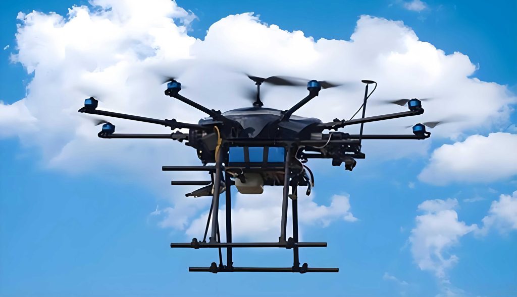
In recent years, the rapid evolution of CNN-based and Transformer-based architectures has transformed the landscape of object detection. CNN-based detectors excel in local feature extraction and computational efficiency, while Transformer-based models demonstrate superior capabilities in modelling long-range dependencies and global contextual information. However, when applied to unmanned aerial vehicles imagery, both paradigms face notable limitations. CNN-based methods often struggle to capture non-local information and suffer from background noise interference. Transformer-based methods, on the other hand, are computationally intensive due to the quadratic complexity of self-attention, which is particularly problematic for high-resolution unmanned aerial vehicles images. Moreover, traditional feature fusion networks used in these detectors mainly focus on aggregating multi-scale features but rarely consider the importance of contextual information surrounding foreground objects. In this thesis, I focus on these problems and propose two novel detection networks specifically designed for aerial imagery of unmanned aerial vehicles.
1 Introduction
With the gradual opening of low-altitude airspace and the rapid advancement of unmanned aerial vehicles technology, intelligent detection algorithms for aerial images have been widely adopted in numerous fields, including smart city construction, traffic monitoring, precision agriculture, environmental protection, disaster assessment, and power infrastructure inspection. Unmanned aerial vehicles equipped with high-resolution cameras can capture imagery from flexible perspectives at varying altitudes, providing a broad field of view and rich spatial information. These characteristics make unmanned aerial vehicles valuable platforms for real-time monitoring and large-scale information acquisition.
However, the object detection task in unmanned aerial vehicles imagery is significantly more challenging than in conventional natural images due to the following factors. First, objects in aerial imagery are usually small in pixel size and occupy only a tiny fraction of the image. Second, backgrounds are complex and may contain texture patterns similar to those of foreground targets, causing severe false positives. Third, target scales vary drastically depending on the flight altitude. These issues aggravate the difficulty of accurate detection and localization.
1.1 Development of Object Detection Technology
Early object detection methods relied heavily on hand-crafted features and shallow machine learning classifiers. Representative works include the Viola-Jones detector, the HOG-based human detector, and the Deformable Part Model (DPM). These methods follow a conventional paradigm of image preprocessing, candidate region generation, hand-crafted feature extraction, and classification. Although these approaches achieved reasonable results in specific tasks, their generalization capability was limited, and they failed when the appearance of objects varied significantly due to changes in viewpoint, illumination, and scale. This limitation is even more severe when processing images captured by unmanned aerial vehicles, where objects often appear at great distances and with relatively poor visual signatures.
The emergence of deep learning, particularly convolutional neural networks, brought about a paradigm shift. In 2012, AlexNet achieved a significant breakthrough in the ImageNet classification competition. This success inspired researchers to apply CNN-based architectures to object detection tasks. As a result, detection frameworks evolved into two major families: two-stage detectors and one-stage detectors.
Two-stage detectors, represented by RCNN, Fast RCNN, Faster RCNN, FPN, and Cascade RCNN, first generate a set of candidate regions and then classify and regress them in a second step. These models generally achieve higher accuracy but at the cost of slower inference speed and higher computational consumption. Faster RCNN, for instance, introduced a Region Proposal Network (RPN) to replace the slow selective search method, enabling end-to-end training and significantly speeding up detection. However, the two-stage pipeline is still less efficient for real-time applications on unmanned aerial vehicles platforms.
One-stage detectors, including the YOLO series, SSD, RetinaNet, and EfficientDet, directly predict object categories and bounding box coordinates from the full image without a separate proposal generation stage. These methods offer a better trade-off between accuracy and speed, making them attractive for real-time unmanned aerial vehicles detection systems. The YOLO family has undergone several iterations from YOLOv1 to YOLO11, each introducing improvements in architecture, feature extraction, and training strategy. Anchor-free approaches such as CenterNet and FCOS remove the reliance on predefined anchor boxes and simplify the detection pipeline. More recently, Transformer-based detectors such as DETR and RT-DETR have challenged conventional designs by treating detection as a set prediction problem and leveraging self-attention for global context modelling.
1.2 Object Detection in Aerial Images of Unmanned Aerial Vehicles
Given the unique properties of unmanned aerial vehicles imagery, many researchers have focused on designing algorithms tailored to this domain. Some methods attempt to improve feature representations for small objects by enriching shallow-level semantics. Others attempt to increase the inference resolution of feature maps to preserve fine-grained details. There are also studies that use attention mechanisms or multi-scale feature fusion to improve the network’s ability to distinguish foreground objects from complex backgrounds. Despite these efforts, many existing algorithms still struggle when evaluating challenging aerial datasets.
In this thesis, I propose two detection algorithms: the Dynamic Context-Guided Network (DCGNet) and the Multi-branch Large Kernel Transformer (MLK-TR). The first algorithm is designed to achieve a balance between accuracy and model complexity, while the second focuses on improving the detection performance in complex aerial scenes. The effectiveness of these algorithms is verified on public benchmark datasets for unmanned aerial vehicles aerial detection, and their practical utility is further validated in a typical application scenario: insulator defect detection on power transmission lines.
2 Foundations and Related Work
This section reviews several mainstream object detection algorithms and attention mechanisms that are relevant to the methods proposed in this thesis.
2.1 Overview of Mainstream Detectors
To provide a comprehensive context for the comparative experiments, I introduce the baseline detectors used in this work. Their main properties and structural characteristics are summarized in Table 1.
| Algorithm | Type | Backbone / Neck | Key Features |
|---|---|---|---|
| EfficientDet | One-stage | EfficientNet / BiFPN | Composite scaling, weighted bi-directional feature fusion |
| YOLOv5 | One-stage | CSPDarknet / PANet | anchor-based, mosaic augmentation, AutoAnchor |
| YOLOX | One-stage | CSPDarknet / PANet | anchor-free, decoupled head, SimOTA label assignment |
| CenterNet | Anchor-free | Hourglass / — | center-point based detection, no anchor |
| FCOS | Anchor-free | ResNet / FPN | pixel-wise regression, centerness branch, multi-scale prediction |
| RT-DETR | Transformer | ResNet / efficient hybrid encoder | real-time DETR, no NMS, mixed-scale attention |
| Faster RCNN | Two-stage | ResNet / FPN | RPN proposal generation, RoI pooling |
2.2 Attention Mechanisms
Attention mechanisms are widely used in object detection to adaptively focus on important features. The SE-Net is one of the pioneering approaches in channel attention. It performs global average pooling, followed by fully connected layers to generate channel-wise weights. The operations can be written as:
$$ z_c = \frac{1}{H \times W} \sum_{i=1}^{H} \sum_{j=1}^{W} X_c(i,j) $$
$$ s = \sigma\left(W_2 \, \delta\left(W_1 z\right)\right) $$
where \(H\) and \(W\) are the height and width of the feature map, \(X_c\) is the \(c\)-th channel of the input feature, \(W_1\) and \(W_2\) are the weights of the two fully connected layers, \(\delta\) is the ReLU function, and \(\sigma\) is the sigmoid function.
The ECA-Net proposes an efficient alternative by using a fast 1D convolution over the channel dimension to model local cross-channel interactions:
$$ s = \sigma\left(\mathrm{Conv1D}_k\left(z\right)\right) $$
where the kernel size \(k\) is adaptively determined according to the channel dimension \(C\):
$$ k = \left\lvert \frac{\log_2 C + b}{\gamma} \right\rvert_{odd} $$
CBAM combines channel attention and spatial attention in a sequential manner, allowing the network to attend to both informative channels and important spatial regions.
However, these attention mechanisms often operate with a limited receptive field. For unmanned aerial vehicles aerial images, a global understanding of the scene is often necessary to distinguish small objects from their highly similar backgrounds.
2.3 Vision Transformer
Vision Transformer (ViT) was the first architecture to apply transformer encoders directly to image patches. The input image is first split into fixed-size patches, then linearly projected into embeddings, and fed into a standard Transformer encoder composed of multi-head self-attention (MHSA) and feed-forward networks. The MHSA operation can be expressed as:
$$ \mathrm{head}_i = \mathrm{softmax}\left(\frac{Q_i K_i^T}{\sqrt{d_k}}\right) V_i $$
$$ \mathrm{MHSA}(Q, K, V) = \mathrm{Concat}(\mathrm{head}_1, \dots, \mathrm{head}_N) W^O $$
where \(Q\), \(K\), \(V\) are the query, key, and value matrices, \(d_k\) is the dimension of the key, \(N\) is the number of heads, and \(W^O\) is a projection matrix. While MHSA provides a powerful mechanism for global interaction, its computation grows quadratically with the number of patches, making it difficult to apply on high-resolution aerial images from unmanned aerial vehicles.
2.4 Benchmark Datasets and Evaluation Metrics
To evaluate the performance of detection algorithms for unmanned aerial vehicles imagery, I adopt two widely used public aerial datasets, namely VisDrone and UAVDT.
The VisDrone dataset is one of the most popular benchmarks for unmanned aerial vehicles object detection. It contains 10209 static images captured by drones from various scenes and altitudes, annotated for 10 object categories, including pedestrians, cars, vans, buses, trucks, motorcycles, bicycles, and tricycles. The UAVDT dataset consists of frames sampled from 100 videos, annotated with three object classes, i.e., car, truck, and bus. In this thesis, I randomly sample 2,000 images from UAVDT for a fair comparison.
Several standard evaluation metrics are used throughout the experiments. Precision (P) reflects the proportion of true positive predictions among all predicted positive samples. Recall (R) denotes the proportion of true positive samples correctly identified. Average precision (AP) summarizes the precision-recall curve for a specific class, while mean average precision (mAP) averages the AP over all classes. Additionally, parameters (Params), computational cost (GFLOPs), and frames per second (FPS) are used to evaluate model complexity and inference efficiency.
3 Dynamic Context-Guided Network for Aerial Image Detection
3.1 Motivation
In Chapter 1, I explained that CNN-based detectors have advantages in extracting local features and achieving fast inference, but they fail to capture non-local information and suppress background noise. Transformer-based models can establish cross-region pixel relationships, but the quadratic complexity of self-attention limits their application to high-resolution unmanned aerial vehicles images. Furthermore, existing feature fusion networks are mostly concerned with multi-scale feature aggregation, while ignoring the surrounding environment of foreground objects which is crucial for accurate localization.
To address these issues, I propose a Dynamic Context-Guided Network (DCGNet), built upon YOLOv8n. The overall architecture of DCGNet is presented in Figure 3.1. DCGNet comprises three main novel components: the Multi-branch Partially Transformer Block (MBPTB), the Dynamic Down-sampling Module (DyDown), and the Context-Guided Feature Fusion Network (CGFFN).
3.2 Multi-branch Partially Transformer Block
The MBPTB is designed to strengthen the model’s ability to extract global features while suppressing background noise. It follows a partial Transformer design, where the input feature map is split into two equal parts along the channel dimension. One part is processed through a Bottleneck branch that captures local features, while the other part is processed by an MHSA-CGLU branch. The CGLU (Convolutional Gated Linear Unit) is used instead of a standard MLP because it preserves details more effectively for small objects.
Given an input feature map \(X_i \in \mathbb{R}^{H \times W \times C_{in}}\), the MBPTB first performs a \(1 \times 1\) convolution to reorganize the features, then splits it as follows:
$$ X_{ptb} = \mathrm{Split}(X_i) \in \mathbb{R}^{H \times W \times C_{out}/2} $$
$$ X_{ptb1}, X_{ptb2} = \mathrm{Split}(X_{ptb}) \in \mathbb{R}^{H \times W \times C_{out}/4} $$
Then the two branch features are processed in parallel:
$$ Y_1 = \mathrm{Bottleneck}(X_{ptb1}) $$
$$ Y_2 = \mathrm{MHSA\text{-}CGLU}(X_{ptb2}) $$
where \(Y_1\) and \(Y_2\) are outputs from the Bottleneck branch and the MHSA-CGLU branch, respectively. Finally, the two parts are concatenated and processed by a \(1 \times 1\) convolution to fuse the features:
$$ Y = \mathrm{Conv}_{1 \times 1}(\mathrm{Concat}(Y_1, Y_2)) $$
This hybrid design enables the model to acquire global dependencies at a lower computation cost, which is beneficial for unmanned aerial vehicles detection tasks.
3.3 Dynamic Down-sampling Module
To mitigate the loss of fine-grained information in traditional down-sampling operations, I propose the DyDown module. The module first applies average pooling to the input feature map, then splits it into two branch features. One branch is processed through a dynamic convolution, and the other branch is processed with a cascaded structure of max pooling and dynamic convolution. The final output is obtained by concatenating the two branch outputs:
$$ H_j = \mathrm{AvgPool}(H_i) $$
$$ H_{b1} = \mathrm{DynamicConv}(H_j[:, :C/2]) $$
$$ H_{b2} = \mathrm{DynamicConv}(\mathrm{MaxPool}(H_j[:, C/2:])) $$
$$ H_o = \mathrm{Concat}(H_{b1}, H_{b2}) $$
where \(H_i\), \(H_j\), and \(H_o\) are the input, intermediate, and output feature maps respectively. This design preserves abundant boundary and location information, which is critical for small object detection in unmanned aerial vehicles aerial imagery. The module also achieves a good trade-off between computational cost and information retention.
3.4 Context-Guided Feature Fusion Network
Traditional feature fusion networks often fail to utilize contextual information around foreground objects. To solve this problem, I design the CGFFN based on the Multi-branch Context-Guided Module (MBCGM). The MBCGM uses a dual-path structure to extract features from both the foreground object itself and its surrounding environment. In the main branch, the CGBlock learns detailed features via a conventional \(3 \times 3\) convolution and contextual features via a dilated \(3 \times 3\) convolution. The two branches are then fused, and a global pooling branch provides a channel-wise weight to enhance useful information:
$$ F_{dilated} = \mathrm{DilatedConv}_{3 \times 3}(F_{main}) $$
$$ F_{conv} = \mathrm{Conv}_{3 \times 3}(F_{main}) $$
$$ F_{fused} = \mathrm{Concat}(F_{conv}, F_{dilated}) $$
$$ F_{weighted} = \mathrm{AvgPool}(F_{fused}) \otimes F_{fused} $$
where \(\otimes\) denotes the multiplication operation. The path-separation strategy enables the model to distinguish defects or objects from similar-texture backgrounds. The CGFFN significantly improves the localization ability of the detector in multi-scale detection scenarios.
3.5 Experimental Results of DCGNet
3.5.1 Implementation Details
All experiments are carried out on an NVIDIA GeForce RTX 3090 24GB GPU with an Intel i9-13900k CPU. The model is trained for 200 epochs with an input size of \(640 \times 640\), a batch size of 16, and the Adam optimizer. The initial learning rate is set to \(1 \times 10^{-3}\), weight decay is \(5 \times 10^{-4}\), and the momentum is set to 0.937.
3.5.2 Comparison with State-of-the-art Methods
Table 3.1 presents a quantitative comparison between DCGNet and other mainstream detectors on the VisDrone and UAVDT datasets. The best results are highlighted in bold.
| Method | VisDrone | UAVDT | Params (M) ↓ | FPS ↑ | |||||
|---|---|---|---|---|---|---|---|---|---|
| P ↑ | R ↑ | mAP50 ↑ | P ↑ | R ↑ | mAP50 ↑ | ||||
| YOLOv3-Tiny | 0.315 | 0.222 | 20.2 | 0.873 | 0.761 | 85.3 | 12.13 | 396 | |
| YOLOv5n | 0.355 | 0.285 | 26.7 | 0.922 | 0.816 | 92.1 | 1.76 | 285 | |
| YOLOv6n | 0.306 | 0.256 | 22.9 | 0.886 | 0.719 | 84.0 | 4.20 | 303 | |
| YOLOv7-Tiny | 0.491 | 0.366 | 35.1 | 0.912 | 0.942 | 96.4 | 6.03 | 340 | |
| YOLOv8n | 0.367 | 0.287 | 27.8 | 0.918 | 0.861 | 94.4 | 3.00 | 300 | |
| YOLOv9t | 0.373 | 0.286 | 27.6 | 0.874 | 0.879 | 93.6 | 1.97 | 147 | |
| YOLOv10n | 0.344 | 0.283 | 25.8 | 0.884 | 0.823 | 91.4 | 2.69 | 222 | |
| YOLO11n | 0.424 | 0.317 | 31.7 | 0.935 | 0.921 | 96.3 | 2.58 | 255 | |
| Hyper-YOLO | 0.422 | 0.317 | 31.8 | 0.933 | 0.901 | 94.6 | 3.94 | 215 | |
| DCGNet | 0.489 | 0.381 | 35.7 | 0.938 | 0.949 | 97.0 | 2.48 | 216 | |
From Table 3.1, it is evident that DCGNet achieves the highest mAP50 on both datasets. On VisDrone, DCGNet achieves a mAP50 of 35.7%, which is 7.9% higher than the baseline YOLOv8n and 4% higher than YOLO11n. On UAVDT, DCGNet achieves the highest mAP50 of 97.0%, with precision and recall values of 0.938 and 0.949, respectively. These results reveal the strong ability of DCGNet in detecting objects under complex aerial scenes. The visual comparison in Figure 3.6 further confirms that DCGNet can reduce false detections and missed detections, especially in scenes with dense small objects and similar background textures.
3.5.3 Ablation Studies of DCGNet
Ablation experiments are conducted on the VisDrone validation set to verify the contribution of each component. Table 3.2 shows the results.
| CGFFN | DyDown | MBPTB | P ↑ | R ↑ | mAP50 ↑ | Params (M) ↓ | FPS ↑ |
|---|---|---|---|---|---|---|---|
| – | – | – | 0.367 | 0.287 | 27.8 | 3.00 | 308 |
| √ | – | – | 0.435 | 0.323 | 32.3 | 2.63 | 281 |
| – | √ | – | 0.418 | 0.317 | 31.2 | 3.00 | 190 |
| – | – | √ | 0.431 | 0.308 | 31.4 | 2.89 | 255 |
| – | √ | √ | 0.444 | 0.322 | 32.5 | 2.90 | 252 |
| √ | √ | √ | 0.489 | 0.381 | 35.7 | 2.48 | 216 |
Each component contributes positively to the final detection accuracy. The complete DCGNet, integrating CGFFN, DyDown, and MBPTB, improves the baseline by 7.9% in mAP50 while reducing the number of parameters by 0.52M. I further compare the proposed MBPTB with several advanced backbone networks, as shown in Table 3.3.
| Backbone | P ↑ | R ↑ | mAP50 ↑ | Params (M) ↓ | FPS ↑ |
|---|---|---|---|---|---|
| Baseline + LSKNet | 0.387 | 0.296 | 28.8 | 5.98 | 104 |
| Baseline + efficientViT | 0.396 | 0.286 | 27.8 | 4.01 | 82 |
| Baseline + HGNetV2 | 0.406 | 0.294 | 29.4 | 2.35 | 290 |
| Baseline + mobilenetv4 | 0.387 | 0.287 | 28.4 | 5.70 | 218 |
| Baseline + RevCol | 0.383 | 0.289 | 28.0 | 2.27 | 198 |
| Baseline + MBPTB | 0.431 | 0.308 | 31.4 | 2.89 | 255 |
Experiments on different neck networks are also conducted, and the results are listed in Table 3.4.
| Neck | P ↑ | R ↑ | mAP50 ↑ | Params (M) ↓ | FPS ↑ |
|---|---|---|---|---|---|
| Baseline + FPN | 0.367 | 0.287 | 27.8 | 3.00 | 308 |
| Baseline + MAFPN | 0.416 | 0.318 | 30.9 | 2.98 | 263 |
| Baseline + BiFPN | 0.424 | 0.322 | 31.5 | 1.99 | 265 |
| Baseline + CGFFN | 0.435 | 0.323 | 32.3 | 2.63 | 281 |
Finally, the contribution of the DyDown module is compared against traditional down-sampling methods, as shown in Table 3.5.
| Down-sampling Module | P ↑ | R ↑ | mAP50 ↑ | Params (M) ↓ |
|---|---|---|---|---|
| Baseline | 0.367 | 0.287 | 27.8 | 3.00 |
| Baseline + V7Sampling | 0.391 | 0.303 | 29.4 | 2.97 |
| Baseline + ADown | 0.412 | 0.313 | 30.1 | 2.94 |
| Baseline + DyDown | 0.418 | 0.317 | 31.2 | 2.98 |
The experimental results prove that each proposed component of DCGNet brings meaningful improvement for unmanned aerial vehicles image detection tasks while maintaining a reasonable computational cost.
4 Multi-branch Large Kernel Transformer for Complex Aerial Scenes
4.1 Motivation
Although DCGNet achieves a good trade-off between accuracy and efficiency, I observe that the detection performance still has large room for improvement, especially in complex scenes where objects are densely packed or extremely small. Therefore, I propose the Multi-branch Large Kernel Transformer (MLK-TR) to further enhance the detection ability in aerial images from unmanned aerial vehicles.
The MLK-TR architecture is built upon YOLO11n and contains four novel components: the Sparse Large Kernel Attention (SLK-Attention), the C3PA2 module, the Frequent Interaction Feature Fusion Network (FIFFN), and an ultra-high resolution prediction feature map.
4.2 Sparse Large Kernel Attention
In aerial images captured by unmanned aerial vehicles, targets may be located far from the camera, and many irrelevant background regions exist. Traditional attention mechanisms often assign computational resources to the entire image, which is inefficient. SLK-Attention solves this problem by focusing only on important regions while using large-kernel convolutions to expand the receptive field.
The SLK-Attention first applies a \(3 \times 3\) average pooling operation:
$$ I’ = \mathrm{AvgPool}_{3 \times 3}(I) $$
Then a large receptive field feature transformation is performed by decomposing 2D convolutions into cascaded 1D convolutions, using depthwise separable convolutions and dilated depthwise separable convolutions:
$$ I” = \mathrm{DConv}_{5 \times 1}\left(\mathrm{DConv}_{1 \times 5}\left(\mathrm{DWConv}_{3 \times 1}\left(\mathrm{DWConv}_{1 \times 3}\left(I’\right)\right)\right)\right) $$
Finally, the output is obtained by combining the transformed feature with a residual connection and applying a Hardswish activation function:
$$ I_{out} = \mathrm{Hardswish}\left(\mathrm{Conv}_{1 \times 1}\left(I”\right) \cdot I’\right) + I’ $$
This sparsification, combined with large-kernel convolutions, reduces the computational burden while preserving the global context, which is essential for detecting small objects in unmanned aerial vehicles images.
4.3 C3PA2 Module
The C3PA2 module combines the C3PA module (C3 + LK-PAB) with the LK-MBAM module. This design allows the detector to select between two computational paths.
First, I introduce the Large Kernel Additive Self-Attention (LKASA), which uses an additive operation to approximate MHSA in a computationally efficient manner:
$$ \mathrm{LKASA}(Q, K, V) = \gamma\left(\omega(Q) + \omega(K)\right) + V $$
where \(\omega(\cdot)\) denotes the Sparse Large Kernel Attention, and \(\gamma(\cdot)\) represents a depthwise convolution operation applied to the fused feature. In LKASA, the dot-product self-attention is replaced by an additive formulation. This design significantly reduces the computational overhead while retaining the ability to model long-range dependencies.
By combining CNN and LK-AB, the LK-PAB block processes the input feature map as follows:
$$ X_1, X_2 = \mathrm{Split}(X) $$
$$ Y = \mathrm{Concat}\left(\mathrm{CNN}(X_1), \; \mathrm{LK\text{-}AB}(X_2)\right) $$
where \(X\) is the input feature map. This partial processing strategy allows the C3PA module to capture both local structural information and global contextual dependencies at a lower computational cost.
The LK-MBAM module further enhances multi-scale feature extraction by splitting the input into multiple branches, processing each with convolutional kernels of different sizes, and then applying SLK-Attention for weighting. The C3PA2 module can switch between C3PA and LK-MBAM based on the task, thereby providing flexibility and scalability for unmanned aerial vehicles detection systems.
4.4 Frequent Interaction Feature Fusion Network
Conventional feature fusion networks often pass deep-level feature maps directly to the fusion stage without adequate transformation. In FIFFN, I first apply \(1 \times 1\) convolution modules to the backbone output feature maps, thus aligning and enhancing the features. Then shallow feature maps are also enhanced before being concatenated with deep feature maps. Finally, skip connections are introduced to fuse features of the same size from the backbone, the up-sampling path, and the down-sampling path.
The fusion process of the \(R2\) prediction layer can be expressed as:
$$ N_3 = \mathrm{C3PA2}\left(\mathrm{Conv}_{1 \times 1}\left(K_3\right) + \mathrm{Upsample}\left(P_2\right)\right) $$
$$ R_2 = \mathrm{C3PA2}\left(K_3 + N_4 + \mathrm{Conv}_{3 \times 3}\left(N_4\right)\right) $$
where \(K_3\) and \(N_4\) denote the corresponding feature maps from the backbone and the fusion network, respectively. By enabling more frequent interactions between features at different levels, FIFFN effectively improves the multi-scale detection capability of the detector on unmanned aerial vehicles imagery.
4.5 Ultra-high Resolution Prediction Feature Map
For unmanned aerial vehicles images, small objects contain limited visual information. In the original YOLO11n, a low-resolution prediction layer of \(20 \times 20\) is used, which may not retain sufficient detail for small object recognition. To remedy this, I remove the low-resolution feature layer and introduce a new ultra-high resolution prediction feature map of \(160 \times 160\). The refined prediction layers are thus of sizes \(160 \times 160\), \(80 \times 80\), and \(40 \times 40\).
The introduction of higher resolution feature maps provides two benefits: first, it preserves the boundary information and fine-grained details of small objects; second, it avoids the information loss associated with low-resolution layers. As a result, the detector can locate and classify small objects more accurately in complex aerial scenes.
4.6 Experimental Results of MLK-TR
4.6.1 Comparison with YOLO Series Models
I first compare MLK-TR with YOLOv8, YOLOv9, YOLOv10, and YOLO11 models of different scales, as shown in Tables 4.1–4.4.
| Method | Params (M) ↓ | FPS ↑ | mAP50 ↑ | F1 ↑ | P ↑ | R ↑ |
|---|---|---|---|---|---|---|
| YOLOv8n | 3.00 | 300 | 27.8 | 0.31 | 0.367 | 0.287 |
| YOLOv8s | 11.12 | 213 | 35.3 | 0.39 | 0.447 | 0.354 |
| YOLOv8m | 25.84 | 109 | 39.5 | 0.43 | 0.507 | 0.381 |
| YOLOv8l | 43.61 | 72 | 42.3 | 0.45 | 0.529 | 0.408 |
| MLK-TR | 3.70 | 165 | 40.7 | 0.43 | 0.507 | 0.390 |
| Method | Params (M) ↓ | FPS ↑ | mAP50 ↑ | F1 ↑ | P ↑ | R ↑ |
|---|---|---|---|---|---|---|
| YOLOv9t | 1.97 | 147 | 27.6 | 0.31 | 0.373 | 0.286 |
| YOLOv9s | 7.17 | 106 | 36.2 | 0.39 | 0.468 | 0.355 |
| YOLOv9m | 20.16 | 83 | 41.1 | 0.44 | 0.516 | 0.397 |
| YOLOv9c | 25.32 | 80 | 42.4 | 0.46 | 0.535 | 0.406 |
| MLK-TR | 3.70 | 165 | 40.7 | 0.43 | 0.507 | 0.390 |
| Method | Params (M) ↓ | FPS ↑ | mAP50 ↑ | F1 ↑ | P ↑ | R ↑ |
|---|---|---|---|---|---|---|
| YOLOv10n | 2.69 | 222 | 25.8 | 0.29 | 0.344 | 0.283 |
| YOLOv10s | 8.04 | 177 | 33.2 | 0.37 | 0.431 | 0.335 |
| YOLOv10m | 16.46 | 105 | 38.4 | 0.41 | 0.473 | 0.379 |
| YOLOv10l | 25.71 | 71 | 41.7 | 0.45 | 0.509 | 0.407 |
| MLK-TR | 3.70 | 165 | 40.7 | 0.43 | 0.507 | 0.390 |
| Method | Params (M) ↓ | FPS ↑ | mAP50 ↑ | F1 ↑ | P ↑ | R ↑ |
|---|---|---|---|---|---|---|
| YOLO11n | 2.58 | 258 | 31.7 | 0.35 | 0.424 | 0.317 |
| YOLO11s | 9.41 | 195 | 38.9 | 0.42 | 0.501 | 0.374 |
| YOLO11m | 20.03 | 110 | 45.5 | 0.48 | 0.559 | 0.434 |
| YOLO11l | 25.28 | 80 | 45.9 | 0.49 | 0.562 | 0.441 |
| MLK-TR | 3.70 | 165 | 40.7 | 0.43 | 0.507 | 0.390 |
It can be observed that MLK-TR achieves a mAP50 of 40.7% with only 3.70M parameters. Compared with the baseline YOLO11n, MLK-TR improves mAP50 by 9.0%. Compared with YOLOv11s, MLK-TR achieves a 1.8% higher mAP50 while using only 39% of the parameters. Compared with YOLOv8l and YOLOv9c, MLK-TR shows a slightly lower mAP50 but achieves significantly higher FPS, which is crucial for real-time processing on unmanned aerial vehicles.
4.6.2 Comparison with Mainstream Detectors
Table 4.5 compares MLK-TR with a wider range of mainstream detection algorithms, including anchor-based, anchor-free, and DETR-based methods.
| Method | VisDrone | UAVDT | Params (M) ↓ | FPS ↑ | |||||
|---|---|---|---|---|---|---|---|---|---|
| P ↑ | R ↑ | mAP50 ↑ | P ↑ | R ↑ | mAP50 ↑ | ||||
| YOLOv3-Tiny | 0.315 | 0.222 | 20.2 | 0.873 | 0.761 | 85.3 | 12.13 | 396 | |
| YOLOv5n | 0.355 | 0.285 | 26.7 | 0.922 | 0.816 | 92.1 | 1.76 | 285 | |
| YOLOv6n | 0.306 | 0.256 | 22.9 | 0.886 | 0.719 | 84.0 | 4.20 | 303 | |
| YOLOv7-Tiny | 0.491 | 0.366 | 35.1 | 0.912 | 0.942 | 96.4 | 6.03 | 340 | |
| YOLOv8n | 0.367 | 0.287 | 27.8 | 0.918 | 0.861 | 94.4 | 3.00 | 300 | |
| YOLOv9t | 0.373 | 0.286 | 27.6 | 0.874 | 0.879 | 93.6 | 1.97 | 147 | |
| YOLOv10n | 0.344 | 0.283 | 25.8 | 0.884 | 0.823 | 91.4 | 2.69 | 222 | |
| YOLO11n | 0.424 | 0.317 | 31.7 | 0.935 | 0.921 | 96.3 | 2.58 | 255 | |
| Hyper-YOLO | 0.422 | 0.317 | 31.8 | 0.933 | 0.901 | 94.6 | 3.94 | 215 | |
| MLK-TR | 0.507 | 0.390 | 40.7 | 0.949 | 0.963 | 98.2 | 3.70 | 165 | |
MLK-TR achieves the best mAP50 on both datasets. It achieves a mAP50 of 40.7% on VisDrone and 98.2% on UAVDT. In particular, the precision on VisDrone reaches 0.507 and the recall is 0.390, both superior to the other methods. These results demonstrate that MLK-TR is highly effective for object detection in unmanned aerial vehicles imagery, especially in complex scenes.
4.6.3 Ablation Studies of MLK-TR
Table 4.6 shows the influence of each component on the baseline detector. The ultra-high resolution prediction feature map, the C3PA2 module, and the FIFFN all contribute to the final improvement.
| High-resolution map | C3PA2 | FIFFN | P ↑ | R ↑ | mAP50 ↑ | Params (M) ↓ | FPS ↑ |
|---|---|---|---|---|---|---|---|
| – | – | – | 0.424 | 0.317 | 31.7 | 2.58 | 258 |
| √ | – | – | 0.458 | 0.357 | 36.4 | 2.48 | 222 |
| – | √ | – | 0.426 | 0.317 | 31.9 | 2.46 | 153 |
| – | – | √ | 0.481 | 0.420 | 40.2 | 3.67 | 164 |
| √ | √ | – | 0.476 | 0.383 | 38.2 | 2.59 | 208 |
| √ | √ | √ | 0.507 | 0.390 | 40.7 | 3.50 | 165 |
The influence of different prediction feature map resolutions is shown in Table 4.7.
| Low-res (20×20) | Mid-res (40×40) | High-res (80×80) | Ultra-res (160×160) | P ↑ | R ↑ | mAP50 ↑ |
|---|---|---|---|---|---|---|
| √ | – | – | — | 0.359 | 0.154 | 16.1 |
| – | √ | – | — | 0.369 | 0.258 | 25.3 |
| – | – | √ | — | 0.412 | 0.312 | 30.6 |
| – | √ | √ | — | 0.411 | 0.314 | 31.1 |
| √ | √ | √ | — | 0.424 | 0.317 | 31.7 |
| — | √ | – | – | 0.416 | 0.284 | 28.0 |
| — | – | √ | – | 0.455 | 0.333 | 33.7 |
| — | – | – | √ | 0.418 | 0.330 | 32.2 |
| — | √ | √ | – | 0.461 | 0.357 | 36.0 |
| — | √ | √ | √ | 0.458 | 0.357 | 36.4 |
The results confirm that replacing low-resolution prediction maps with the ultra-high resolution \(160 \times 160\) feature map yields a significant improvement in mAP50. The proposed feature extraction modules in C3PA2 are also evaluated, as shown in Table 4.8.
| Module | Params (M) ↓ | GFLOPs ↓ | FPS ↑ |
|---|---|---|---|
| C3k (baseline) | 0.34 | 0.28 | 106 |
| C3PA (MLK-TR) | 0.36 | 0.28 | 88 |
| BottleNeck (baseline) | 0.11 | 0.36 | 83 |
| LK-MBAM (MLK-TR) | 0.06 | 0.21 | 113 |
Furthermore, I compare the backbone integrated with C3PA2 against several widely used lightweight backbone networks. The quantitative results are shown in Table 4.9.
| Method | P ↑ | R ↑ | mAP50 ↑ | Params (M) ↓ | FPS ↑ |
|---|---|---|---|---|---|
| Baseline + LSKNet | 0.385 | 0.292 | 28.2 | 5.62 | 102 |
| Baseline + efficientViT | 0.399 | 0.283 | 28.1 | 3.73 | 104 |
| Baseline + HGNetV2 | 0.386 | 0.303 | 29.1 | 2.14 | 256 |
| Baseline + mobilenetv4 | 0.360 | 0.288 | 26.8 | 5.43 | 236 |
| Baseline + RevCol | 0.360 | 0.271 | 25.8 | 2.09 | 161 |
| Baseline + MLK-TR | 0.452 | 0.348 | 35.3 | 2.41 | 220 |
Finally, the neck networks are compared, and the results are presented in Table 4.10.
| Neck | P ↑ | R ↑ | mAP50 ↑ | Params (M) ↓ | FPS ↑ |
|---|---|---|---|---|---|
| Baseline + FPN | 0.424 | 0.317 | 31.7 | 2.58 | 258 |
| Baseline + MAFPN | 0.430 | 0.325 | 32.2 | 2.68 | 227 |
| Baseline + BiFPN | 0.415 | 0.317 | 30.8 | 1.92 | 217 |
| Baseline + FIFFN | 0.481 | 0.420 | 40.2 | 3.67 | 164 |
In summary, the FIFFN enhances the recall rate more effectively than other feature fusion networks, significantly reducing missed detections. The three proposed components are complementary: the ultra-high resolution map preserves fine-grained details, the C3PA2 module strengthens the global and local feature extraction, and the FIFFN improves the interaction across feature levels. Together, these components enable MLK-TR to achieve state-of-the-art detection accuracy for unmanned aerial vehicles aerial images while maintaining high inference efficiency.
5 Application in Insulator Defect Detection for Power Transmission Lines
5.1 Background and Dataset Construction
To evaluate the practical value of the proposed algorithms, I apply them to a typical industrial scenario: insulator defect detection using unmanned aerial vehicles in power transmission line inspection. Insulators are critical components of power systems, and their defects can cause severe electrical failures. Traditional manual inspection is costly and dangerous. Therefore, using unmanned aerial vehicles equipped with high-resolution cameras to automatically detect insulator defects is of significant practical importance.
In this study, a DJI Matrice 300 RTK unmanned aerial vehicle equipped with a Zenmuse H20T camera is used to collect images of insulators in real transmission line scenes. Finally, 2,150 images with various types of insulator defects are selected. These images contain nine defect categories: glass damage, glass missing, polymer damage, polymer dirt, two-piece glass, breakage, crack, flashover, and snow cover.
The dataset is randomly divided into training, validation, and test subsets. The same experimental setting as in Section 3.5.1 is used for training.
5.2 Experimental Results and Discussion
Table 5.1 and Figure 5.4 report the quantitative comparison results on the insulator defect dataset.
| Method | P ↑ | R ↑ | mAP50 ↑ | FPS ↑ | Params (M) ↓ |
|---|---|---|---|---|---|
| CenterNet | 0.667 | 0.172 | 39.5 | 65 | 32.66 |
| EfficientDet-d1 | 0.420 | 0.170 | 26.8 | 23 | 3.83 |
| RT-DETR | 0.410 | 0.434 | 42.4 | 87 | 8.33 |
| FCOS | 0.554 | 0.467 | 57.2 | 56 | 32.13 |
| YOLOX-Tiny | 0.572 | 0.557 | 62.0 | 110 | 54.21 |
| YOLOv3-Tiny | 0.577 | 0.511 | 50.1 | 394 | 12.13 |
| YOLOv5n | 0.592 | 0.541 | 49.8 | 292 | 1.76 |
| YOLOv6n | 0.533 | 0.491 | 46.8 | 306 | 4.23 |
| YOLOv7-Tiny | 0.621 | 0.573 | 54.5 | 340 | 6.03 |
| YOLOv8n | 0.726 | 0.499 | 51.0 | 308 | 3.00 |
| YOLOv9t | 0.713 | 0.507 | 53.1 | 151 | 1.97 |
| YOLOv10n | 0.551 | 0.438 | 45.7 | 270 | 2.26 |
| YOLOv11n | 0.526 | 0.509 | 52.0 | 260 | 2.58 |
| DCGNet | 0.641 | 0.588 | 56.3 | 216 | 2.48 |
| MLK-TR | 0.680 | 0.620 | 64.2 | 165 | 3.70 |
MLK-TR achieves the highest mAP50 of 64.2%, with a recall of 62.0% and a precision of 68.0%. Compared with the baseline YOLO11n, MLK-TR improves mAP50 by 12.2%. DCGNet also achieves strong results, with an mAP50 of 56.3%, while using only 2.48M parameters. These results confirm that both DCGNet and MLK-TR have excellent generalization ability and practical value in real-world detection tasks involving unmanned aerial vehicles.
The visual comparison in Figure 5.5 further demonstrates that MLK-TR and DCGNet can accurately locate defects and reduce false positives even under conditions of low contrast and complex backgrounds. These advantages originate from the improved feature extraction and fusion capabilities of the proposed modules.
6 Conclusion and Outlook
In this thesis, I address the key challenges of object detection in aerial images captured by unmanned aerial vehicles. The main contributions can be summarized as follows.
First, I propose the Dynamic Context-Guided Network (DCGNet), which integrates three major components: the Multi-branch Partially Transformer Block (MBPTB), the Dynamic Down-sampling Module (DyDown), and the Context-Guided Feature Fusion Network (CGFFN). The MBPTB enhances the global feature extraction capability while suppressing background noise. The DyDown module preserves edge information during down-sampling and improves the model’s ability to detect small objects. The CGFFN enables the model to learn both object features and contextual features, thereby improving its robustness in complex scenes. Extensive experiments on the VisDrone and UAVDT datasets demonstrate that DCGNet achieves a good trade-off between accuracy and efficiency.
Second, I propose the Multi-branch Large Kernel Transformer (MLK-TR). This network introduces the Sparse Large Kernel Attention (SLK-Attention) mechanism to reduce computational overhead and enhance global information capture. The C3PA2 module allows for flexible switching between two powerful feature extraction paths and effectively captures multi-scale features. The Frequent Interaction Feature Fusion Network (FIFFN) promotes dense information interaction across feature levels, while the ultra-high resolution prediction feature map maintains fine-grained details for small object detection. MLK-TR achieves state-of-the-art performance on both benchmark datasets, demonstrating its strong capability in complex aerial detection scenarios.
Finally, I apply the proposed algorithms to the task of insulator defect detection using unmanned aerial vehicles. Experimental results show that both DCGNet and MLK-TR outperform mainstream detectors in terms of mAP50, demonstrating their strong industrial applicability and generalization potential.
Although the proposed methods achieve significant progress, there is still room for future improvement. First, future research could explore the fusion of multi-source data, such as infrared images, RGB images, and LiDAR data, to further improve detection accuracy and robustness. Second, the multi-scale object detection problem, especially small object detection in unmanned aerial vehicles imagery, deserves further investigation. Third, model compression techniques such as quantization, pruning, and knowledge distillation could be applied to meet the real-time constraints of resource-limited unmanned aerial vehicles platforms. Finally, weakly supervised or self-supervised learning methods could be considered to reduce the dependence on large-scale labeled data, which is often costly to obtain for aerial scenes.