
Unmanned aerial vehicles (UAVs) have become indispensable tools in a wide range of civil and military applications, including environmental monitoring, precision agriculture, infrastructure inspection, search and rescue, and battlefield reconnaissance. The ability to navigate autonomously in the absence of global navigation satellite system (GNSS) signals is a critical requirement for many of these missions. In GNSS-denied environments such as deep mountain canyons, dense forests, urban canyons, indoor spaces, and electronic warfare zones, the satellite signals are often blocked, interfered, or spoofed, making traditional navigation systems unreliable or completely unavailable. Consequently, research on robust, self-contained navigation technologies for unmanned aerial vehicles has attracted increasing attention worldwide.
This paper presents a complete autonomous navigation system for four-rotor unmanned aerial vehicles that relies on stereo vision and inertial measurement unit (IMU) fusion. I focus on two core modules: (1) a visual simultaneous localization and mapping (SLAM) framework that improves the robustness of pose estimation and achieves real-time three-dimensional (3D) mapping; and (2) a fast path planning algorithm that combines a modified Informed-RRT* method with the dynamic window approach (DWA) to handle both static and dynamic obstacles in complex 3D environments. The proposed system is validated using the EuRoC public dataset, simulation experiments, and real-world flight tests, demonstrating significant improvements in localization accuracy, mapping quality, and planning efficiency compared with baseline methods.
The key contributions of this work are summarized as follows:
- I propose a point-line feature fusion visual-inertial SLAM system based on the ORB-SLAM3 framework. An improved LSD line segment detector with length filtering and segment merging is designed to extract high-quality line features. A fast binocular line triangulation method is proposed to achieve efficient and accurate 3D reconstruction of line features without relying on expensive descriptor matching.
- I introduce a refined line reprojection error model that uses the midpoint distance and angular difference between the projected line and the observed line segment. By combining point and line features in a unified nonlinear optimization framework with Huber robust kernels, the proposed method significantly improves the pose estimation accuracy in low-texture environments.
- I present an efficient approach for real-time 3D mapping using an octree-based occupancy grid. The dense depth maps from the stereo camera are integrated into a probabilistic octree representation, enabling memory-efficient storage and fast updates of the environment model, which is directly suitable for UAV navigation.
- I develop a hybrid path planning algorithm that integrates an improved Informed-RRT* with the dynamic window approach. The global planner generates a collision-free reference path, while the local DWA controller performs real-time obstacle avoidance and trajectory optimization. The proposed algorithm reduces path length, planning time, and the number of redundant nodes in both static and dynamic environments.
1. Introduction
Autonomous navigation of unmanned aerial vehicles in GNSS-denied environments is a challenging problem that has attracted significant research interest. Traditional satellite-based navigation systems rely heavily on line-of-sight signals from space, which are vulnerable to physical blockage, electromagnetic interference, and deliberate spoofing. In contrast, vision-based navigation using onboard cameras offers a low-cost, passive, and information-rich alternative. Modern visual SLAM techniques allow a UAV to simultaneously estimate its pose and build a map of the surrounding environment, which is essential for safe and efficient path planning.
However, several technical challenges remain. First, in low-texture or poorly illuminated scenes, feature point extraction often fails, causing visual SLAM systems to lose tracking or diverge. Second, conventional sparse point cloud maps are insufficient for path planning because they do not explicitly encode free and occupied spaces. Third, path planning in 3D space requires algorithms that can handle high-dimensional state spaces while satisfying the dynamic constraints of the UAV.
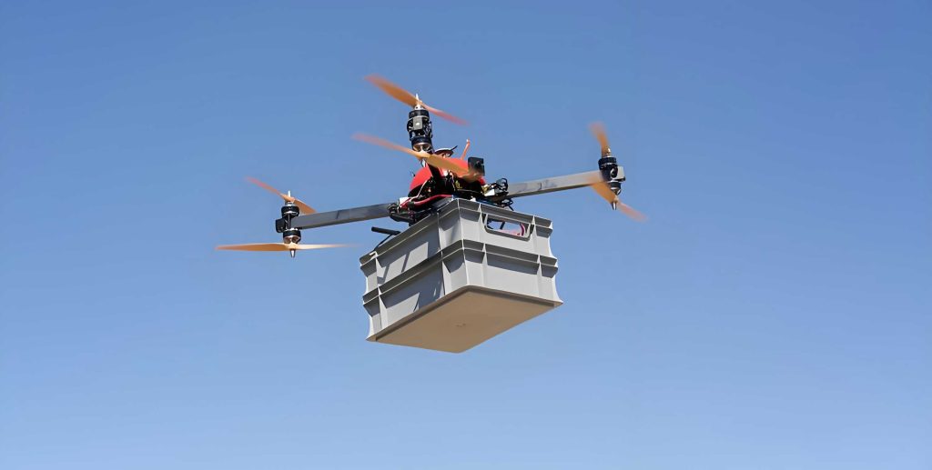
To address these challenges, I developed a complete autonomous navigation pipeline for unmanned aerial vehicles, integrating advanced visual-inertial SLAM with a novel path planning strategy. The overall architecture of the proposed system is illustrated conceptually in the following figure, which shows a UAV operating in a complex outdoor environment with obstacles.
2. System Design and Problem Modeling
2.1 Overall System Architecture
The proposed autonomous navigation system consists of four interconnected modules: perception, localization and mapping, motion planning, and control. The perception module uses a stereo camera and an IMU to capture raw sensory data. The localization and mapping module performs visual-inertial odometry to estimate the UAV pose and builds an octree-based 3D occupancy map. The motion planning module receives the map and target waypoint, generates a collision-free global path, and then refines it locally using the DWA. Finally, the control module sends actuator commands to the flight controller to follow the planned trajectory.
The system is designed to operate in real-time on embedded computing platforms such as the NVIDIA Jetson series, which provides sufficient computational power for processing stereo images and running the SLAM and planning algorithms.
2.2 Visual SLAM Model
Visual SLAM estimates the ego-motion of a camera and constructs a representation of the environment from image sequences. A standard visual SLAM system consists of front-end (visual odometry), back-end (optimization), loop closure, and mapping modules. In this work, I adopt the ORB-SLAM3 framework as the base system because it supports monocular, stereo, and RGB-D cameras, integrates IMU measurements in a tightly-coupled manner, and provides robust place recognition and multi-map capabilities. However, ORB-SLAM3 relies purely on point features, which makes it less robust in low-texture environments. Therefore, I enhance the front-end by adding line features to improve tracking stability and map richness.
2.3 UAV Localization Problem Formulation
The UAV state at discrete time step \(k\) is represented by a vector \(\mathbf{x}_k\) that includes position, velocity, orientation, and sensor biases. The motion of the UAV is modeled as a nonlinear state transition:
\[
\mathbf{x}_k = f(\mathbf{x}_{k-1}, \mathbf{u}_k, \mathbf{w}_k)
\]
where \(\mathbf{u}_k\) is the control input from the IMU (linear acceleration and angular velocity), and \(\mathbf{w}_k\) represents the process noise. The observation model relates the UAV state to the sensor measurements:
\[
\mathbf{z}_{k,j} = h(\mathbf{y}_j, \mathbf{x}_k) + \mathbf{v}_{k,j}
\]
where \(\mathbf{y}_j\) is the \(j\)-th landmark in the environment, and \(\mathbf{v}_{k,j}\) is the measurement noise. The goal of localization is to estimate the posterior distribution \(p(\mathbf{x}_k | \mathbf{z}_{1:k}, \mathbf{u}_{1:k})\). In this work, I use a graph-based nonlinear optimization formulation to minimize the sum of squared reprojection errors for both point and line observations.
2.4 Stereo Camera Model
The stereo camera consists of two identical cameras separated by a baseline \(b\). The geometric relation for a 3D point \(P\) observed by both cameras is expressed by the disparity \(d = u_L – u_R\), which is inversely proportional to the depth \(z\):
\[
z = \frac{f \cdot b}{d}
\]
where \(f\) is the focal length. Accurate calibration of intrinsic parameters and distortion coefficients is essential for reliable depth computation. I use a standard pin-hole model with radial and tangential distortion correction, as described in the following equations:
\[
x’ = x (1 + k_1 r^2 + k_2 r^4 + k_3 r^6) + 2 p_1 x y + p_2 (r^2 + 2 x^2)
\]
\[
y’ = y (1 + k_1 r^2 + k_2 r^4 + k_3 r^6) + p_1 (r^2 + 2 y^2) + 2 p_2 x y
\]
where \(r^2 = x^2 + y^2\), \((x,y)\) are normalized coordinates, and \((k_1, k_2, k_3, p_1, p_2)\) are the distortion coefficients.
2.5 Hardware Platform
To validate the proposed algorithms, I built a quadrotor UAV platform with the following components:
| Component | Specification |
|---|---|
| Frame | Q250 carbon-fiber chassis, 250 mm wheelbase |
| Motors | TMOTOR V2306-2400KV brushless motors |
| Propellers | GEMFAN 51477 5-inch |
| ESC | HSKRC 45A |
| Battery | TATTU 4S 2300 mAh LiPo |
| Flight controller | CUAV V5 nano (Pixhawk FMUv5) with built-in IMU |
| Onboard computer | NVIDIA Jetson NX |
| Stereo camera | Orbbec DaBai DCW (1920×1080, 30 FPS, 0.2–2.5 m) |
The onboard computer handles all perception, mapping, and planning computations. The flight controller is responsible for low-level attitude and rate control, while the onboard computer sends high-level velocity or position commands via MAVROS.
3. Point-Line Feature Fusion for UAV Localization and Mapping
3.1 Proposed Visual-Inertial SLAM Framework
The proposed visual-inertial SLAM system extends ORB-SLAM3 by integrating line features into the tracking, local mapping, and optimization stages. The overall architecture consists of four threads: (1) front-end feature extraction and tracking, (2) local mapping, (3) loop closure, and (4) octree mapping. In the front-end, I detect ORB keypoints and line segments in parallel. The line detector is an improved version of LSD (Line Segment Detector) that includes length filtering and segment merging to produce more stable and meaningful line features. Stereo matching of line features is performed using a geometric-constrained method that exploits the epipolar geometry of the parallel stereo rig.
3.2 Improved LSD Line Feature Extraction
LSD is an efficient line segment detector that uses the gradient orientation information to produce subpixel-accurate lines. However, raw LSD outputs many short and fragmented segments that are not suitable for robust matching. I improve the algorithm by applying the following steps:
- Sorting: All detected line segments are sorted in descending order of their length.
- Short-line removal: A length threshold \(l_{\min}\) is defined as \(l_{\min} = \delta \cdot \min(M, N)\), where \(M,N\) are the image dimensions and \(\delta\) is a scaling factor (set to 0.07 through experiments). Segments shorter than this threshold are discarded.
- Angle filtering: Candidate segments whose orientation differs from the orientation of the longest segment by less than an angle threshold \(\theta_{\min}\) are retained. The angle difference is computed in a computationally efficient way using horizontal and vertical distances.
- Segment merging: Adjacent nearly-collinear segments are merged into longer segments, which improves stability and reduces redundancy.
The effectiveness of the improved LSD algorithm is evaluated on the EuRoC dataset. The results show that the number of extracted line features is reduced by about 50% while the average line length increases by 80%, leading to better matching performance and lower computational cost.
3.3 Fast Binocular Line Triangulation
Traditional line triangulation relies on the LBD descriptor to match line features between left and right images, which is computationally expensive and suffers from low recall in low-texture scenes. Instead, I propose a geometric-constrained stereo matching method that exploits the parallel-axis stereo configuration. The matching cost between a candidate line pair \((l_i^m, l_j^m)\) is defined as a weighted combination of four terms:
\[
\mathbf{Q}_{ij} = \begin{bmatrix} E_{ij}^p \\ D_{ij} \\ N_{ij} \\ U_{ij} \end{bmatrix}
\]
where \(E_{ij}^p\) is the parallel error based on the cosine of the angle between the two segments:
\[
E_{ij}^p = 1 – \cos(l_i^m, l_j^m)
\]
\(D_{ij}\) is the distance between the endpoints in the horizontal direction (epipolar constraint), \(N_{ij}\) is derived from the normalized cross-correlation (NCC) of the local intensity patches around the segment midpoints, and \(U_{ij}\) is the length ratio error. The optimal matching is obtained by solving an L1-regularized least-squares problem, which yields a sparse solution indicating the best match.
After matching, the endpoints of the left line are projected onto the right image along epipolar lines, and the intersections with the right matched line are computed to obtain the corresponding endpoints. The 3D line is then reconstructed by back-projecting the matched endpoints.
3.4 Line Reprojection Error and Pose Optimization
The pose estimation is formulated as a nonlinear optimization that minimizes the sum of point and line reprojection errors. For point features, the reprojection error is the Euclidean distance between the projected 3D point and the observed 2D keypoint:
\[
\mathbf{e}_{k,i}^p = \mathbf{p}’_{k,i} – \pi(\mathbf{R}_{k}^{k-1} \mathbf{P}_i + \mathbf{t}_{k}^{k-1})
\]
where \(\pi(\cdot)\) is the projection function, and \(\mathbf{R}, \mathbf{t}\) are the rotation and translation to be optimized.
For line features, I propose an improved error model that uses the Manhattan distance between the midpoint of the observed line segment and the projected infinite line, as well as the angle difference between the two lines. Let \(\mathbf{l}_c\) be the projected line in the normalized image plane, and let \((\bar{x}, \bar{y})\) be the midpoint of the observed segment. The line reprojection residual is defined as:
\[
\mathbf{e}_{k,j}^l = \begin{bmatrix} d \\ \theta \end{bmatrix}
\]
where \(d = |l_1 \bar{x} + l_2 \bar{y} + l_3|\) is the Manhattan distance (normalized by the line coefficients) and
\[
\theta = \arctan\left( \frac{k_{\text{obs}} – k_{\text{proj}}}{1 + k_{\text{obs}} k_{\text{proj}}} \right)
\]
with \(k_{\text{obs}}\) and \(k_{\text{proj}}\) being the slopes of the observed and projected lines, respectively. This model is simpler and more robust than the conventional endpoint-based error because it does not require exact endpoint correspondences.
The full optimization problem is
\[
\mathbf{T}^* = \arg\min_{\mathbf{T}} \sum_{i \in \mathcal{P}} \rho_H \left( \mathbf{e}_{k,i}^{p\top} \boldsymbol{\Omega}^p \mathbf{e}_{k,i}^p \right) + \sum_{j \in \mathcal{L}} \rho_H \left( \mathbf{e}_{k,j}^{l\top} \boldsymbol{\Omega}^l \mathbf{e}_{k,j}^l \right)
\]
where \(\rho_H\) is the Huber robust loss function, and \(\boldsymbol{\Omega}^p, \boldsymbol{\Omega}^l\) are the information matrices for point and line measurements, respectively. The Huber kernel is defined as
\[
\rho_H(e) = \begin{cases} 0.5 e^2, & \text{if } |e| \le \delta \\ \delta(|e| – 0.5 \delta), & \text{otherwise} \end{cases}
\]
This formulation effectively reduces the influence of outlier measurements. The optimization is solved using the Levenberg-Marquardt algorithm embedded in g2o or GTSAM.
3.5 Real-Time Octree-Based 3D Mapping
To support UAV navigation, I construct a 3D occupancy grid map using an octree representation. The octree algorithm recursively subdivides a cubic space into eight sub-cubes. Each leaf node stores the probability that the corresponding volume is occupied. The probability is updated using a log-odds formulation:
\[
L(n) = \log \left( \frac{p(n)}{1 – p(n)} \right)
\]
The log-odds update rule for a measurement \(z_t\) is
\[
L(n | z_{1:t}) = L(n | z_{1:t-1}) + L(n | z_t)
\]
This allows fast incremental updates as the UAV moves. The stereo depth map is back-projected to a point cloud and integrated into the octree map. The resulting map explicitly distinguishes free, occupied, and unknown spaces, which is essential for collision checking in path planning. Furthermore, the octree representation is memory-efficient because it only subdivides regions that contain occupied cells or are ambiguous, while large free regions are represented by a single node.
I tested the mapping algorithm on the EuRoC MH_03 sequence. The RGB image and depth map were processed online, and the resulting octree map accurately captured the geometry of the indoor machine hall. The map resolution was set to 0.05 m, and the update rate was about 10 Hz, which met the real-time requirements.
4. Fast Path Planning for UAVs
4.1 Problem Formulation
Let \(\mathcal{X} \subset \mathbb{R}^3\) be the 3D workspace. Denote by \(\mathcal{X}_{\text{obs}}\) the obstacle region and \(\mathcal{X}_{\text{free}} = \mathcal{X} \setminus \mathcal{X}_{\text{obs}}\) the free space. A path planning problem is defined as finding a continuous function \(\sigma: [0,1] \to \mathcal{X}_{\text{free}}\) such that \(\sigma(0) = x_{\text{start}}\), \(\sigma(1) = x_{\text{goal}}\), and \(\sigma(\tau) \in \mathcal{X}_{\text{free}}\) for all \(\tau \in [0,1]\). The objective is to minimize the path cost \(c(\sigma)\), which is typically the Euclidean length of the path.
4.2 RRT* and Informed-RRT*
The Rapidly-exploring Random Tree (RRT) algorithm is a popular sampling-based planner that builds a tree by randomly sampling the free space. RRT* improves upon RRT by introducing two additional steps: choosing the parent node that minimizes the cost-to-come, and rewiring the tree to maintain asymptotic optimality. The key steps of RRT* are summarized in the following pseudocode:
| Algorithm 1: RRT* |
|---|
| 1: \(V \leftarrow \{x_{\text{start}}\}, E \leftarrow \emptyset\) 2: for \(i = 1\) to MaxIter do 3: \(x_{\text{rand}} \leftarrow \text{Sample}()\) 4: \(x_{\text{near}} \leftarrow \text{Nearest}(V, x_{\text{rand}})\) 5: \(x_{\text{new}} \leftarrow \text{Steer}(x_{\text{near}}, x_{\text{rand}})\) 6: if \(\text{CollisionFree}(x_{\text{near}}, x_{\text{new}})\) then 7: \(X_{\text{near}} \leftarrow \text{Near}(V, x_{\text{new}})\) 8: \(x_{\text{parent}} \leftarrow \text{ChooseParent}(X_{\text{near}}, x_{\text{near}}, x_{\text{new}})\) 9: \(V \leftarrow V \cup \{x_{\text{new}}\}\) 10: \(E \leftarrow E \cup \{(x_{\text{new}}, x_{\text{parent}})\}\) 11: \(\text{Rewire}(G, X_{\text{near}}, x_{\text{new}})\) 12: end if 13: end for 14: return \(G = (V,E)\) |
Informed-RRT* refines RRT* by focusing the sampling on an elliptical region defined by the current best path cost \(c_{\text{best}}\). The ellipse has foci at the start and goal points, and its semi-major axis is \(c_{\text{best}}/2\). This sampling strategy significantly accelerates convergence by avoiding unnecessary exploration outside the promising region.
4.3 Improved Informed-RRT* with APF
Despite its advantages, Informed-RRT* still suffers from large number of redundant nodes and long planning time in complex environments. I propose two modifications:
(1) Adaptive Goal Biasing
I introduce an adaptive factor \(\alpha \in [0,1]\) that depends on the distance between the start and goal:
\[
\alpha = 1 – \frac{\| x_{\text{goal}} – x_{\text{start}} \|}{n}
\]
where \(n\) is a normalization constant. The random sample is generated according to
\[
x_{\text{rand}} = \begin{cases} x_{\text{goal}}, & \text{with probability } \alpha \cdot \beta \\ \text{Uniform}(\mathcal{X}_{\text{free}}), & \text{otherwise} \end{cases}
\]
where \(\beta\) is a control parameter. This strategy gives a higher probability of sampling toward the goal when the path is shorter, improving convergence.
(2) APF-Guided Node Expansion
In the standard RRT* expansion, the new node \(x_{\text{new}}\) is generated along the direction from \(x_{\text{near}}\) to \(x_{\text{rand}}\). I modify this by adding attractive and repulsive forces similar to the Artificial Potential Field (APF) method. The attractive force from the goal and the random sample, and the repulsive force from nearby obstacles, collectively determine the expansion direction. The combined force is
\[
F_{\text{total}} = F_{\text{att},1} + F_{\text{att},2} + F_{\text{rep}}
\]
where
\[
F_{\text{att},1} = k_a \frac{x_{\text{goal}} – x_{\text{near}}}{\| x_{\text{goal}} – x_{\text{near}} \|}
\]
\[
F_{\text{att},2} = k_b \frac{x_{\text{rand}} – x_{\text{near}}}{\| x_{\text{rand}} – x_{\text{near}} \|}
\]
and
\[
F_{\text{rep}} = \begin{cases} k_r \left( \frac{1}{d} – \frac{1}{Q} \right) \frac{x_{\text{near}} – x_{\text{obs}}}{d^2}, & \text{if } d \le Q \\ 0, & \text{otherwise} \end{cases}
\]
Here, \(k_a, k_b, k_r\) are weighting coefficients, \(d = \| x_{\text{near}} – x_{\text{obs}} \|\) is the distance to the nearest obstacle, and \(Q\) is the influence range of obstacles. The new node is then placed as
\[
x_{\text{new}} = x_{\text{near}} + \frac{F_{\text{total}}}{\|F_{\text{total}}\|} \cdot S
\]
where \(S\) is the step size. This reduces the randomness of the tree growth and keeps the sampling away from obstacles, resulting in fewer redundant nodes and faster convergence.
4.4 Path Smoothing
The path generated by the improved Informed-RRT* is still piecewise linear and may contain sharp turns that are not flyable for a quadrotor. I apply cubic spline interpolation to generate a smooth trajectory. The spline passes through all the waypoints and respects the curvature constraint. The curvature at a point is computed as
\[
\kappa(t) = \frac{|x'(t) y”(t) – y'(t) x”(t)|}{(x'(t)^2 + y'(t)^2)^{3/2}}
\]
To ensure the UAV can follow the path, the curvature is limited by the maximum turning rate defined by the vehicle dynamics. If the curvature exceeds the limit, the interpolation points are adjusted by a scaling factor to reduce the curvature.
4.5 Dynamic Window Approach (DWA) for Local Avoidance
Although the global path is collision-free with respect to the known map, unexpected obstacles may appear in the environment. To handle these dynamic or unknown obstacles, I integrate the Dynamic Window Approach (DWA) as a local planner. DWA performs velocity sampling in the robot’s motion space and evaluates each candidate trajectory using a cost function:
\[
G(v, w) = \alpha \cdot \text{heading}(v, w) + \beta \cdot \text{obsdist}(v, w) + \gamma \cdot \text{velocity}(v, w) + \delta \cdot \text{smoothness}(a)
\]
where \(\text{heading}\) measures the angular difference to the goal, \(\text{obsdist}\) measures the distance to the nearest obstacle along the trajectory, \(\text{velocity}\) encourages forward motion, and \(\text{smoothness}\) penalizes large accelerations. The DWA algorithm runs at a high frequency (20–50 Hz) and only considers velocities that are reachable within a short time window, which ensures real-time responsiveness.
The integration of Informed-RRT* and DWA works as follows: the global planner computes a reference path from the start to the goal. The DWA tracker then attempts to follow this path while performing local repairs when unexpected obstacles are detected. The output of the DWA is a set of velocity commands that are sent to the flight controller.
5. Simulation and Experimental Results
5.1 Evaluation of Pose Estimation Accuracy
I evaluate the proposed visual-inertial SLAM system on the EuRoC dataset, which provides synchronized stereo images and IMU data recorded on a micro aerial vehicle. The dataset includes ground truth pose trajectories measured by a Vicon motion capture system. I selected the MH_03 sequence for detailed comparison. The absolute pose error (APE) is used as the metric:
\[
\text{APE} = \sqrt{\frac{1}{N} \sum_{i=1}^{N} \| \text{trans}(\mathbf{T}_{\text{est},i}^{-1} \mathbf{T}_{\text{gt},i}) \|^2}
\]
| Algorithm | Max (m) | Min (m) | Std (m) | Median (m) | Mean (m) | RMSE (m) |
|---|---|---|---|---|---|---|
| ORB-SLAM3 | 0.091 | 0.004 | 0.015 | 0.028 | 0.031 | 0.035 |
| Proposed method | 0.081 | 0.002 | 0.014 | 0.020 | 0.025 | 0.029 |
The proposed method achieves a 17.14% reduction in RMSE compared with ORB-SLAM3, confirming that the integration of line features improves the accuracy of pose estimation, especially in structured indoor environments with repetitive textures.
5.2 3D Mapping Results
Using the EuRoC MH_03 dataset, I successfully built an octree-based 3D occupancy map. The stereo depth images were fused with the optimized pose estimates to create a dense reconstruction. The octree map resolution was set to 0.05 m, and the resulting map accurately represented walls, pillars, and other structures. The map was suitable for direct use in collision checking for path planning.
I also performed real-time mapping on the onboard computer during flight tests. The system maintained an update rate of approximately 10 Hz while running both localization and mapping concurrently, demonstrating its practical viability.
5.3 Path Planning Simulation
I compared the proposed improved Informed-RRT* algorithm with the standard RRT* and Informed-RRT* in three different environments: (A) general open space, (B) narrow corridor-like space, and (C) cluttered environment. Each environment is 100 m × 100 m. The UAV is modeled as a point with a minimum turning radius constraint. To account for the randomness of sampling-based algorithms, each experiment was repeated 30 times.
The following tables summarize the average results for each environment.
Environment A (General)
| Algorithm | Avg nodes | Time (s) | Avg path length (m) | Success rate |
|---|---|---|---|---|
| RRT* | 566 | 8.9856 | 127.3167 | 80% |
| Informed-RRT* | 524 | 7.3331 | 119.7200 | 83% |
| Proposed | 126 | 1.3452 | 115.0886 | 93% |
Environment B (Narrow)
| Algorithm | Avg nodes | Time (s) | Avg path length (m) | Success rate |
|---|---|---|---|---|
| RRT* | 572 | 8.2394 | 125.5162 | 76% |
| Informed-RRT* | 506 | 7.4856 | 123.7842 | 83% |
| Proposed | 167 | 1.8220 | 115.4792 | 90% |
Environment C (Cluttered)
| Algorithm | Avg nodes | Time (s) | Avg path length (m) | Success rate |
|---|---|---|---|---|
| RRT* | 486 | 6.3901 | 128.7113 | 86% |
| Informed-RRT* | 437 | 5.9795 | 127.1665 | 90% |
| Proposed | 155 | 1.6915 | 117.8026 | 93% |
The proposed algorithm significantly reduces the number of nodes and planning time, while improving the success rate and shortening the path length. This improvement is particularly noticeable in cluttered environments where the APF-guided expansion prevents the tree from growing near obstacles, thus avoiding many collision checks and unnecessary branches.
5.4 Dynamic Obstacle Avoidance
To test the integration with DWA, I added moving obstacles to the simulation environments. The DWA algorithm used the globally planned path as a reference and successfully avoided the moving obstacles while keeping the UAV close to the reference path. The overall flight behavior was smooth, and the UAV reached the goal without collisions. Compared with using only Informed-RRT* (which cannot react to moving obstacles), the fused approach demonstrated clear advantages in dynamic environments.
5.5 Real-World Flight Tests
I integrated the proposed navigation system on the quadrotor platform and conducted experiments in an outdoor courtyard with artificial obstacle gates. The UAV was operated without any GNSS signals, relying solely on the stereo camera and IMU. The on-board computer performed real-time SLAM and path planning, while the Pixhawk controller executed the velocity commands.
During the experiment, the UAV successfully navigated from a start point to a target point while avoiding static obstacles (gate structures) and a moving obstacle (a person walking through the area). The entire process was autonomous with no human intervention. The estimated trajectory and the corresponding map were recorded and visualized in ROS/rviz. The flight trajectory was smooth and stable, and the position error with respect to the planned path was within a few centimeters. This real-world validation demonstrates the practicality and reliability of the proposed system.
6. Conclusion and Future Work
In this paper, I presented a complete autonomous navigation system for quadrotor unmanned aerial vehicles in GNSS-denied environments. The system integrates a point-line feature fusion visual-inertial SLAM with an improved path planning algorithm and a local dynamic obstacle avoidance mechanism. The following conclusions can be drawn from this research:
- The proposed visual SLAM algorithm, which combines ORB point features with improved LSD line features, significantly enhances the robustness and accuracy of pose estimation in low-texture environments. The experimental results on the EuRoC dataset show a 17% reduction in RMSE compared with ORB-SLAM3.
- The octree-based 3D mapping method provides a memory-efficient and navigation-ready representation of the environment. The map can be updated in real time using stereo depth data, making it suitable for online path planning.
- The improved Informed-RRT* algorithm with APF-guided expansion and adaptive sampling drastically reduces the number of nodes, the planning time, and the path length compared with the standard variants. The success rate is also improved due to the more efficient exploration.
- The integration of DWA with the global planner enables the UAV to react to unknown static and dynamic obstacles in real time, preserving a safe and smooth flight path.
- Real-world experiments confirmed that the overall system is capable of autonomous navigation in a GNSS-denied environment without human intervention, achieving stable flight and reliable obstacle avoidance.
There are several directions for future research. First, the current visual SLAM system is sensitive to drastic illumination changes and strong motion blur. Deep learning-based feature extraction and matching methods could be explored to improve robustness. Second, the path planning algorithm currently assumes the UAV is a point mass; incorporating full dynamics constraints, such as minimum turning radius and maximum acceleration, would yield more flyable trajectories. Third, multi-modal sensor fusion (e.g., adding a downward-facing depth sensor or a 2D LiDAR) could further improve the perception reliability. Finally, extending the system to multi-UAV cooperative navigation is an interesting avenue for complex missions.
In summary, this work provides an effective and complete solution for autonomous navigation of unmanned aerial vehicles in challenging GNSS-denied environments, with significant improvements in localization accuracy, mapping efficiency, and path planning performance. The outcomes of this research have immediate applications in search and rescue, inspection, and autonomous delivery using unmanned aerial vehicles.