
In this thesis, I investigate the integration of unmanned aerial vehicles (unmanned aerial vehicles) with extremely large-scale multiple-input multiple-output (XL-MIMO) systems, focusing on two fundamental problems: (i) joint altitude optimization and user scheduling for a UAV-mounted XL-MIMO base station serving multiple ground users, and (ii) beam tracking for a high-mobility UAV served by a ground XL-MIMO base station. Both problems are studied under the near-field spherical-wave propagation regime, which becomes indispensable when the antenna aperture is large enough to extend the Rayleigh distance to tens or hundreds of meters. I first derive a set of orthogonal positions for users in the near-field region of a uniform planar array (UPA), based on the maximum achievable sum-rate criterion. Using these orthogonal positions, I propose a user scheduling algorithm and a particle-swarm-optimization (PSO) based altitude search algorithm. Simulation results show significant sum-rate gains over existing far-field baseline methods. Then, for the downlink from a ground XL-MIMO array to a moving UAV, I propose a beam tracking method that minimizes the variance of the beam gain over the UAV’s predicted trajectory. The UAV position is estimated via an extended Kalman filter (EKF) using the spherical-wave phase difference measurements. A near-field codebook is employed to select quantization points covering the predicted motion range, and a phase-parameter optimization problem is solved by PSO. Numerical results demonstrate that the proposed beamformer maintains a stable received signal-to-noise ratio (SNR) and achieves higher average rate than conventional matched-filter (MF) fixed-beam and gradient-phase wide-beam approaches.
1. Introduction
The fifth-generation (5G) mobile communication system has been deployed worldwide, yet its limitations in coverage depth, spectral efficiency, and energy efficiency motivate the development of the sixth-generation (6G) system. Among the key enabling technologies for 6G, unmanned aerial vehicles (unmanned aerial vehicles) and extremely large-scale MIMO (XL-MIMO) have attracted intensive research interest. UAVs provide flexible deployment, strong line-of-sight (LoS) links, and three-dimensional (3D) mobility, making them ideal platforms for temporary base stations, relays, and edge computing nodes. On the other hand, XL-MIMO, which employs hundreds or thousands of antennas, offers unprecedented spatial resolution and array gain, enabling high spectral efficiency and precise beam focusing. However, the combination of these two technologies introduces new challenges due to the near-field effect. When the antenna aperture is large, the Rayleigh distance \(r_{\mathrm{Rayleigh}} = 2D^2/\lambda\) (where \(D\) is the array aperture and \(\lambda\) is the wavelength) can reach tens or hundreds of meters. A UAV flying close to such an array lies in the near-field region, where the conventional planar-wave assumption fails, and spherical-wave propagation must be adopted. This fundamentally changes the channel model, the design of codebooks, and the optimization of UAV positions. Most existing works on UAV communication with massive MIMO assume far-field planar-wave channels. In contrast, this thesis addresses the near-field scenario and develops new solutions for UAV position optimization and beam tracking.
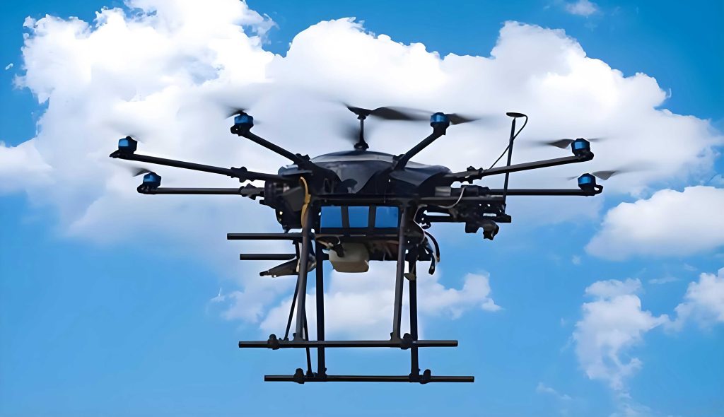
The contributions of this thesis can be summarized as follows. First, I consider a downlink communication system where a UAV equipped with an XL-MIMO UPA serves multiple single-antenna users. I derive a set of user orthogonal positions in the near-field region, characterized by both angular and distance coordinates, such that the channel vectors of different users are mutually orthogonal. This orthogonality eliminates inter-user interference and maximizes the achievable sum-rate. Based on these positions, I propose a user scheduling algorithm that selects the most suitable users to move to orthogonal positions, and a PSO-based altitude optimization algorithm to find the best UAV height. Second, I study the beam tracking problem for a high-speed UAV communicating with a ground XL-MIMO array. I employ an EKF to estimate the UAV position from the spherical-wave phase differences. The predicted motion range is then used to determine the beam coverage in angle and distance domains. A near-field codebook is used to select quantization points within the coverage, and a beamforming vector is designed to minimize the variance of the beam gain. PSO optimizes the phase parameters. Extensive simulations verify the effectiveness of the proposed algorithms.
2. System Models and Near-Field Channel
2.1 UAV-Mounted XL-MIMO Downlink System
As shown in the system model in this thesis, a UAV acts as an aerial base station equipped with a UPA of \(M = M_x \times M_y\) antennas, where \(M_x\) and \(M_y\) are the number of antennas along the \(x\)- and \(y\)-axes, respectively. The antenna spacing is \(d = \lambda/2\). A set of \(K\) single-antenna users is located on the sea surface (or ground). The UAV hovers at altitude \(H\), and its projection on the ground is taken as the origin of the \(xyz\) coordinate system. The position of the \(k\)-th user is denoted by \(\mathbf{q}_k = [x_k, y_k, H]^T\), and its spherical coordinates are \((r_k, \theta_k, \phi_k)\), where \(r_k\) is the radial distance from the first antenna, \(\theta_k\) is the elevation angle, and \(\phi_k\) is the azimuth angle. The transformation is \(x_k = r_k \sin\theta_k \cos\phi_k\), \(y_k = r_k \sin\theta_k \sin\phi_k\), and \(z_k = H = r_k \cos\theta_k\).
Since the UAV is in the near-field of the UPA, the channel vector is modeled by spherical waves. The channel between the UAV and the \(k\)-th user is written as
$$
\mathbf{h}_k = \frac{\lambda}{4\pi r_k} e^{-j\frac{2\pi}{\lambda} r_k} \mathbf{a}(r_k, \theta_k, \phi_k),
$$
where \(\mathbf{a}(r_k, \theta_k, \phi_k)\) is the near-field array response vector:
$$
\mathbf{a}(r_k, \theta_k, \phi_k) = \frac{1}{\sqrt{M}} \left[ e^{-j\frac{2\pi}{\lambda} (r_k^{(0)} – r_k)}, e^{-j\frac{2\pi}{\lambda} (r_k^{(1)} – r_k)}, \ldots, e^{-j\frac{2\pi}{\lambda} (r_k^{(M-1)} – r_k)} \right]^T,
$$
and \(r_k^{(m)}\) is the distance from the \(k\)-th user to the \(m\)-th antenna. For a UPA with the \(m\)-th antenna located at \((i_m d, j_m d, 0)\), the distance is given by
$$
r_k^{(m)} = \sqrt{ r_k^2 + (i_m d)^2 + (j_m d)^2 – 2 r_k d (i_m \sin\theta_k \cos\phi_k + j_m \sin\theta_k \sin\phi_k) }.
$$
The received signal at the \(k\)-th user is
$$
y_k = \sqrt{\rho} \, \mathbf{h}_k^H \mathbf{w}_k s_k + \sum_{j \neq k} \sqrt{\rho} \, \mathbf{h}_k^H \mathbf{w}_j s_j + n_k,
$$
where \(\rho = P/\sigma^2\) is the transmit SNR, \(P\) is the total transmit power, \(\sigma^2\) is the noise power, \(s_k\) is the data symbol for user \(k\) with unit power, \(\mathbf{w}_k\) is the beamforming vector, and \(n_k \sim \mathcal{CN}(0,1)\). I adopt maximum-ratio transmission (MRT) beamforming:
$$
\mathbf{w}_k = \frac{\mathbf{h}_k}{\|\mathbf{h}_k\|}.
$$
The achievable sum-rate is
$$
R = \sum_{k=1}^{K} \log_2 \left( 1 + \frac{\rho |\mathbf{h}_k^H \mathbf{w}_k|^2}{\rho \sum_{j \neq k} |\mathbf{h}_k^H \mathbf{w}_j|^2 + 1} \right).
$$
2.2 Ground XL-MIMO Serving a UAV
In the second scenario, a ground base station with an XL-MIMO UPA serves a single-antenna UAV. The UAV moves with a high speed, and the base station needs to track its beam continuously. The UAV position at time \(t\) is denoted by \(\mathbf{p}(t) = [x(t), y(t), z(t)]^T\) or equivalently in spherical coordinates \(\mathbf{p}(t) = [r(t), \theta(t), \phi(t)]^T\). The channel vector is similarly given by the near-field spherical-wave model. The received signal at the UAV is
$$
y(t) = \sqrt{\rho} \, \mathbf{h}^H(t) \mathbf{f}(t) s(t) + n(t),
$$
where \(\mathbf{f}(t) \in \mathbb{C}^{M \times 1}\) is the beamforming vector with \(\|\mathbf{f}(t)\|=1\). The beam gain at the UAV position is defined as
$$
\gamma(\mathbf{p}(t)) = |\mathbf{a}^H(\mathbf{p}(t)) \mathbf{f}(t)|^2.
$$
3. User Orthogonal Positions in the Near Field
The key to maximizing the sum-rate is to eliminate inter-user interference. From the singular value decomposition of the channel matrix, the maximum sum-rate is achieved when the user channels are mutually orthogonal. Therefore, I aim to find a set of positions such that \(\mathbf{h}_p^H \mathbf{h}_q = 0\) for all \(p \neq q\). Starting from the channel expression, the inner product is
$$
\mathbf{h}_p^H \mathbf{h}_q = \frac{\lambda^2}{16\pi^2 r_p r_q} e^{j\frac{2\pi}{\lambda}(r_p – r_q)} \mathbf{a}^H(r_p,\theta_p,\phi_p) \mathbf{a}(r_q,\theta_q,\phi_q).
$$
Thus, orthogonality requires
$$
\mathbf{a}^H(r_p,\theta_p,\phi_p) \mathbf{a}(r_q,\theta_q,\phi_q) = 0.
$$
To solve this, I approximate the distance \(r^{(m)}\) using the Fresnel approximation and a decoupling of the cross terms. The resulting phase in the sum can be separated into an angular part and a distance-dependent part. The angular part is analogous to the far-field DFT codebook condition, while the distance part is solved using the Fresnel integral approximation. The complete derivation yields a set of orthogonal positions parameterized by a layer index \(s\) and an angle index \(n\).
Theorem 1 (Orthogonal positions for a UPA). Given an \(M_x \times M_y\) UPA with wavelength \(\lambda\) and antenna spacing \(d\), there exists a set of orthogonal positions \(\mathcal{P} = \{\mathbf{p}_n^{(s)}\}\) such that any two users placed on different positions have orthogonal channels. The positions are given in spherical coordinates as
$$
\mathbf{p}_n^{(s)} = [r_{s,n}, \theta_n, \phi_n]^T,
$$
where
$$
\phi_n = \arctan \left( \frac{(2m_y – 1) M_y – M_x}{(2m_x – 1) M_x – M_y} \right),
$$
$$
\theta_n = \arcsin \left( \sqrt{ \left( \frac{2m_x – 1 – M_x}{d M_x \lambda} \right)^2 + \left( \frac{2m_y – 1 – M_y}{d M_y \lambda} \right)^2 } \right),
$$
and the distance is either
$$
r_{s,n} = \frac{Z_{x,\Delta}}{s} \left( 1 – 2 \sin^2\theta_n \cos^2\phi_n \right)^{-1} \quad \text{or} \quad
r_{s,n} = \frac{Z_{y,\Delta}}{s} \left( 1 – 2 \sin^2\theta_n \sin^2\phi_n \right)^{-1},
$$
with \(Z_{x,\Delta} = d^2 M_x^2 \lambda \beta_\Delta / 2\), \(Z_{y,\Delta} = d^2 M_y^2 \lambda \beta_\Delta / 2\), and \(\beta_\Delta\) a constant threshold. Here \(m_x \in \mathcal{M}_x\), \(m_y \in \mathcal{M}_y\) satisfy the feasible range constraints, \(s \in \{1,2,\ldots,S\}\), \(n = 1,\ldots,N\), and \(N = M_x \times M_y\).
This theorem generalizes several known results. When the array reduces to a uniform linear array (ULA) with \(d = \lambda/2\), it recovers the near-field polar-domain sampling grid of the spatial sparsity transform. When the distance tends to infinity, it recovers the far-field angular orthogonality condition \(\sin\theta_p \cos\phi_p – \sin\theta_q \cos\phi_q = n/(d M_x)\). For a UPA, the far-field orthogonal positions correspond to the classical DFT beamforming grid.
Since users are constrained to lie on the sea surface (or ground plane), their height is fixed at \(z = H\). Therefore, not all orthogonal positions are accessible. I developed Algorithm 1 to generate the set of sea-level orthogonal positions from the full 3D set.
| Algorithm 1: Sea-level orthogonal position generation |
|---|
|
Input: array dimensions \(M_x, M_y\), wavelength \(\lambda\), antenna spacing \(d\), threshold \(\beta_\Delta\), altitude \(H\), tolerance \(\Delta_H\). Output: set \(\mathcal{P}_{\mathrm{sea}} = \{\mathbf{p}_1,\ldots,\mathbf{p}_L\}\). 1. Compute \(Z_{x,\Delta}, Z_{y,\Delta}\). 2. For each layer \(s\) and each valid angle index \(n\), compute \(\mathbf{p}_n^{(s)}\) from Theorem 1. 3. Convert to Cartesian coordinates \(\mathbf{p}_n^{(s)} = [x, y, z]^T\). 4. If \(z \in [H – \Delta_H, H + \Delta_H]\), add \(\mathbf{p}_n^{(s)}\) to \(\mathcal{P}_{\mathrm{sea}}\). 5. Remove duplicates and sort by layer. 6. Return \(\mathcal{P}_{\mathrm{sea}}\). |
4. UAV Altitude Optimization and User Scheduling
4.1 Problem Formulation
Given the set of sea-level orthogonal positions, the optimization problem is to choose which users should move to which orthogonal positions, and to find the optimal UAV altitude \(H\), so that the achievable sum-rate is maximized. The problem is formulated as
$$
\max_{H, \{b_{k,l}\}} R(H, \{b_{k,l}\})
$$
$$
\text{s.t. } b_{k,l} \in \{0,1\}, \sum_{l=1}^L b_{k,l} \le 1, \sum_{k=1}^K b_{k,l} \le 1, \quad H_{\min} \le H \le H_{\max},
$$
where \(b_{k,l}=1\) indicates that user \(k\) is assigned to orthogonal position \(l\). The problem is non-convex due to the binary variables and the nonlinear dependence of \(R\) on positions.
4.2 User Scheduling Algorithm
When the number of users \(K\) exceeds the number of available orthogonal positions \(L\), not all users can be moved to interference-free locations. I propose an interference-aware scheduling algorithm (ICIBS) that first selects the \(L\) users with the strongest mutual interference, assigns them to the orthogonal positions using the Hungarian algorithm, and leaves the remaining users at their original positions. The interference metric for user \(k\) is defined as
$$
\iota_k = \sum_{j \neq k} \frac{|\mathbf{h}_k^H \mathbf{h}_j|^2}{\|\mathbf{h}_k\|^2 \|\mathbf{h}_j\|^2}.
$$
The algorithm selects the \(L\) users with the largest \(\iota_k\) and then solves an assignment problem to minimize the total movement distance while maximizing the sum-rate. This is particularly effective when the number of orthogonal positions is limited by the altitude and array configuration.
| Algorithm 2: User scheduling based on interference selection |
|---|
|
Input: user positions, \(\mathcal{P}_{\mathrm{sea}}\), channel vectors. Output: assignment matrix \(\mathbf{B}\). 1. Compute \(\iota_k\) for all users. 2. If \(K > L\), select the \(L\) users with the largest \(\iota_k\); otherwise select all users. 3. Build a cost matrix based on the Euclidean distance between selected users and orthogonal positions. 4. Apply the Hungarian algorithm to find the optimal assignment. 5. Set \(b_{k,l}\) accordingly. 6. Return \(\mathbf{B}\). |
4.3 PSO-based Altitude Optimization
Since the altitude \(H\) affects the number of sea-level orthogonal positions, the assignment, and the channel gains, I use a particle swarm optimization (PSO) algorithm to search for the optimal altitude. Each particle represents a candidate altitude \(H\). For each particle, the scheduling algorithm is executed, and the sum-rate is evaluated. The PSO updates the particle velocities and positions using the standard rules:
$$
v_{q}^{(t+1)} = w v_{q}^{(t)} + c_1 r_1 (U_{q,\mathrm{best}}^{(t)} – U_q^{(t)}) + c_2 r_2 (U_{\mathrm{global}}^{(t)} – U_q^{(t)}),
$$
$$
U_q^{(t+1)} = U_q^{(t)} + v_{q}^{(t+1)},
$$
where \(w\) is the inertia weight, \(c_1, c_2\) are acceleration coefficients, \(r_1, r_2\) are uniform random numbers, \(U_{q,\mathrm{best}}\) is the personal best altitude, and \(U_{\mathrm{global}}\) is the global best altitude. The algorithm iterates until convergence and returns the optimal altitude \(H_{\mathrm{opt}}\) and the corresponding user assignment.
5. UAV Beam Tracking in Near Field
5.1 UAV Motion Model and EKF
In the beam tracking scenario, the UAV moves continuously. The state vector at the beginning of the \(k\)-th frame is \(\mathbf{c}_k = [\mathbf{p}_k^T, \mathbf{v}_k^T]^T\), where \(\mathbf{v}_k = [v_{x,k}, v_{y,k}, v_{z,k}]^T\) is the velocity. The state evolution is
$$
\mathbf{c}_k = \mathbf{A} \mathbf{c}_{k-1} + \mathbf{n}_k,
$$
with
$$
\mathbf{A} = \begin{bmatrix} \mathbf{I}_3 & T_f \mathbf{I}_3 \\ \mathbf{0}_3 & \mathbf{I}_3 \end{bmatrix},
$$
where \(T_f\) is the frame duration, and \(\mathbf{n}_k \sim \mathcal{N}(0, \mathbf{Q})\) is the process noise. The covariance matrix is
$$
\mathbf{Q} = \begin{bmatrix} \frac{T_f^3}{3} \mathbf{Q}_a & \frac{T_f^2}{2} \mathbf{Q}_a \\ \frac{T_f^2}{2} \mathbf{Q}_a & T_f \mathbf{Q}_a \end{bmatrix},
$$
with \(\mathbf{Q}_a = \mathrm{diag}(\sigma_{a,x}^2, \sigma_{a,y}^2, \sigma_{a,z}^2)\).
The measurement vector is the set of phase differences between different antennas and the reference antenna:
$$
\mathbf{z}_k = \mathbf{g}(\mathbf{p}_k) + \mathbf{n}_k^p,
$$
where \(\mathbf{g}_m(\mathbf{p}_k) = \frac{2\pi}{\lambda} (r_k^{(m)} – r_k) \mod 2\pi\). Since \(\mathbf{g}\) is nonlinear, the EKF is used. The Jacobian matrix \(\mathbf{G}_k = \nabla_{\mathbf{p}} \mathbf{g}(\mathbf{p})|_{\mathbf{p}=\hat{\mathbf{p}}_k}\) is computed analytically. The EKF equations are as follows:
$$
\hat{\mathbf{c}}_{k|k-1} = \mathbf{A} \hat{\mathbf{c}}_{k-1|k-1},
$$
$$
\mathbf{P}_{k|k-1} = \mathbf{A} \mathbf{P}_{k-1|k-1} \mathbf{A}^T + \mathbf{Q},
$$
$$
\mathbf{K}_k = \mathbf{P}_{k|k-1} \mathbf{G}_k^T (\mathbf{G}_k \mathbf{P}_{k|k-1} \mathbf{G}_k^T + \mathbf{R})^{-1},
$$
$$
\hat{\mathbf{c}}_{k|k} = \hat{\mathbf{c}}_{k|k-1} + \mathbf{K}_k (\mathbf{z}_k – \mathbf{g}(\hat{\mathbf{p}}_{k|k-1})),
$$
$$
\mathbf{P}_{k|k} = (\mathbf{I} – \mathbf{K}_k \mathbf{G}_k) \mathbf{P}_{k|k-1}.
$$
The EKF provides a smoothed position estimate at the current frame and a predicted position for the next frame. The predicted position \(\mathbf{p}^+ = \mathbf{p}_{k+1|k}\) is then used to design the beam coverage.
5.2 Beam Coverage Determination
Given the current estimated position \(\mathbf{p}^- = [r^-, \theta^-, \phi^-]^T\) and the predicted next-frame position \(\mathbf{p}^+ = [r^+, \theta^+, \phi^+]^T\), the beam must cover the entire region between these two points during the frame duration. Since the UAV moves with a bounded acceleration, the true position at any time within the frame lies in an ellipsoidal uncertainty region. Using the 3\(\sigma\) principle, I define the elevation coverage interval as
$$
\Theta = [\theta_c – 2\delta_\theta, \theta_c + 2\delta_\theta],
$$
where \(\theta_c = (\theta^+ + \theta^-)/2\) and \(\delta_\theta = \max(3\sigma_{\theta^-}, 3\sigma_{\theta^+})\). Similarly, the azimuth coverage is \(\Phi = [\phi_c – 2\delta_\phi, \phi_c + 2\delta_\phi]\). For the distance domain, the near-field codebook has discrete layers. I identify the layer indices \(s^-\) and \(s^+\) that enclose \(r^-\) and \(r^+\), respectively, and set the distance coverage from layer \(s_{\min} = \min(s^-, s^+)\) to \(s_{\max} = \max(s^-, s^+) + 1\). The selected quantization points are those whose elevation, azimuth, and layer indices fall within the corresponding intervals.
5.3 Beamforming Design
The proposed beamforming vector is a linear combination of the near-field array response vectors corresponding to the selected quantization points:
$$
\mathbf{f} = \frac{1}{\sqrt{L}} \sum_{l=1}^{L} e^{j \eta_l} \mathbf{a}(r_l, \theta_l, \phi_l),
$$
where \(L\) is the number of selected quantization points and \(\eta_l \in [0, 2\pi)\) are phase parameters to be optimized. The objective is to minimize the variance of the beam gain over the continuous set of positions inside the coverage region \(\mathcal{C}\). Since the continuous region is difficult to optimize, I sample it with \(U\) points \(\{\mathbf{p}_u\}_{u=1}^U\). The variance is defined as
$$
\mathrm{Var}(\gamma) = \frac{1}{U} \sum_{u=1}^{U} \left( |\mathbf{a}^H(\mathbf{p}_u) \mathbf{f}|^2 – \bar{\gamma} \right)^2,
$$
where \(\bar{\gamma} = \frac{1}{U} \sum_{u=1}^{U} |\mathbf{a}^H(\mathbf{p}_u) \mathbf{f}|^2\). The phase optimization problem is
$$
\min_{\{\eta_l\}} \mathrm{Var}(\gamma)
$$
$$
\text{s.t. } 0 \le \eta_l < 2\pi, \quad l = 1,\ldots,L.
$$
This problem is non-convex, and I solve it with PSO. Each particle represents the vector of phases. The fitness function is the beam-gain variance. The algorithm updates the phases iteratively until convergence.
| Algorithm 3: PSO-based phase optimization |
|---|
|
Input: quantization points \(\{(r_l,\theta_l,\phi_l)\}\), coverage samples \(\{\mathbf{p}_u\}\), PSO parameters. Output: optimized phases \(\{\eta_l\}\). 1. Initialize a population of \(Q\) particles with random phases in \([0, 2\pi)\). 2. For each particle, compute the beamforming vector and evaluate the variance over all sample points. 3. Update personal best and global best. 4. Update particle velocities and positions using the PSO rule. 5. Repeat until the maximum number of iterations or convergence. 6. Return the global best phase vector. |
6. Simulation Results and Analysis
6.1 Simulation Setup for the UAV-Mounted XL-MIMO System
The simulation parameters are summarized in Table 1. The UAV carries a UPA with \(M_x = 250\) and \(M_y = 20\) antennas, i.e., a total of 5000 antennas. The carrier frequency is \(f = 30\) GHz, the antenna spacing is \(d = 5\) mm, and the altitude range is from 10 m to 200 m. The number of users is \(K = 120\) in the sum-rate versus SNR simulation, but I also vary the number of users in another experiment. The transmit SNR \(\rho = P/\sigma^2\) ranges from 80 dB to 120 dB in the comparison, and a fixed \(\rho = 110\) dB is used for the altitude and user-number curves.
| Parameter | Value |
|---|---|
| \(M_x\) | 250 |
| \(M_y\) | 20 |
| Carrier frequency \(f\) | 30 GHz |
| Antenna spacing \(d\) | 5 mm |
| Number of users \(K\) | 120 (variable) |
| Altitude range | [10 m, 200 m] |
| \(\beta_\Delta\) | 1.2 |
| Transmit SNR \(\rho\) | 80–120 dB |
Figure 1 in the original thesis shows a snapshot of the initial user positions and the optimal assignment based on Algorithm 2 when the UAV altitude is 100 m and there are 25 users. The sea-level orthogonal positions are marked, and the users assigned to those positions move there, while other users stay unchanged. This visual result confirms the scheduling behavior.
Figure 2 shows the number of sea-level orthogonal positions and the achievable sum-rate as functions of the UAV altitude. The number of orthogonal positions first increases and then decreases with altitude. This is caused by the balance between the expanding footprint and the reduced spatial resolution in the distance domain. The sum-rate follows a similar trend, indicating that the UAV altitude directly affects the inter-user interference reduction. The optimal altitude is around 120 m in this setting.
Figure 3 compares the sum-rate versus transmit SNR for four schemes: (1) proposed full scheme (orthogonal positions + ICIBS scheduling + PSO altitude), (2) users stay at initial positions with only altitude optimization, (3) Hungarian scheduling without interference selection, and (4) a discrete search algorithm for altitude. The proposed scheme achieves the highest sum-rate over the entire SNR range. The gain is particularly large when the SNR is high, because the inter-user interference becomes the dominant limiting factor, and the orthogonal positions eliminate this interference.
Figure 4 plots the sum-rate versus the number of users at \(\rho = 110\) dB. When the user number is below the number of orthogonal positions (around 90), all scheduling algorithms perform almost identically because every user can be assigned to an orthogonal position. When the user number exceeds this threshold, the proposed ICIBS selection significantly outperforms both the fixed-position and the Hungarian-only methods. This demonstrates the robustness of the scheduling algorithm in overloaded scenarios.
Figure 5 shows the convergence behavior of the PSO altitude optimization. The sum-rate increases rapidly during the first 10 iterations and becomes stable after about 22 iterations, confirming that the algorithm converges reliably.
6.2 Simulation Setup for the UAV Beam Tracking System
The beam tracking simulation parameters are listed in Table 2. The ground base station uses a UPA of \(M_x = 250\) and \(M_y = 50\) antennas, with the same carrier frequency of 30 GHz. The transmit SNR is 100 dB. The frame duration is \(T_f = 1\) s, and each frame has \(\Gamma = 10\) time slots. The UAV initial state is \(\mathbf{c}_0 = [1, 0.5, 21, 0.97, 0, 1]^T\), with velocities in m/s. The process noise variances are \(\sigma_{a,x}^2 = 0.1\), \(\sigma_{a,y}^2 = 0\), and \(\sigma_{a,z}^2 = 0.1\) (in m/s\(^2\) units appropriately scaled). The initial covariance is \(\mathbf{P}_0 = \mathrm{diag}(0.25, 0.25, 0.01, 0.09409, 0, 0.01)\).
| Parameter | Value |
|---|---|
| \(M_x\) | 250 |
| \(M_y\) | 50 |
| Carrier frequency \(f\) | 30 GHz |
| Transmit SNR \(\rho\) | 100 dB |
| Number of frames \(K\) | 10 |
| Slots per frame \(\Gamma\) | 10 |
| Frame duration \(T_f\) | 1 s |
| Initial state \(\mathbf{c}_0\) | \([1, 0.5, 21, 0.97, 0, 1]^T\) |
| Process noise \(\mathbf{Q}_a\) | diag(0.1, 0, 0.1) |
| \(\mathbf{P}_0\) | diag(0.25, 0.25, 0.01, 0.09409, 0, 0.01) |
Figure 6 (in the original thesis) shows the true UAV trajectory, the predicted positions from the state evolution model, and the EKF-estimated positions. The EKF estimates are much closer to the true trajectory than the open-loop predictions, confirming the necessity of the update step.
Figure 7 shows the effect of the number of sample points \(U\) on the beam-gain variance. The variance decreases as \(U\) increases, but the marginal gain diminishes after \(U = 60\). Therefore, I choose \(U = 60\) as a trade-off between performance and complexity.
Figure 8 plots the received SNR of the UAV over time for three beam tracking approaches: (a) the fixed beam based on MF pointing to the current estimated position at the start of a frame, (b) the gradient-phase wide-beam method from the far-field literature, and (c) the proposed near-field PSO-phase beamformer. The fixed-beam SNR drops sharply within each frame because the UAV moves away from the narrow beam. The gradient-phase method provides a wider beam but still exhibits non-negligible fluctuation. The proposed method maintains a nearly constant SNR, indicating that the beam coverage matches the UAV motion range and the gain is flat over the coverage.
Figure 9 shows the average achievable rate per frame. The proposed method achieves the highest average rate in every frame, followed by the gradient-phase method, and the fixed-beam method has the lowest rate. These results validate the effectiveness of the proposed near-field beam tracking design.
Figure 10 demonstrates the convergence of the PSO phase optimization for three representative frames. In all cases, the variance decreases monotonically and converges within about 30 iterations, proving the stability of the algorithm.
7. Discussion and Future Work
This thesis has provided a comprehensive framework for integrating unmanned aerial vehicles with extremely large-scale MIMO in near-field propagation environments. The derived orthogonal positions are particularly useful for multi-user UAV-mounted base stations, as they transform the interference channel into a set of parallel independent channels. The scheduling and altitude optimization algorithms exploit the new distance domain of near-field XL-MIMO to maximize the sum-rate. In the beam tracking scenario, the EKF-based position estimation combined with the near-field codebook and PSO-phase optimization provides a robust solution for maintaining a stable link to a fast-moving UAV. Compared to far-field adaptive beamforming, the near-field method takes into account the spherical wavefront, leading to a much flatter beam gain over a 3D volume.
There are several possible extensions of this work. First, the user scheduling algorithm can be extended to a multi-cell scenario where multiple UAV base stations cooperate. Second, the beam tracking method can be generalized to multiple UAVs or to UAVs with multiple antennas, which will require joint spatial-temporal processing. Third, the spherical-wave model can be refined to include non-uniform spherical waves when the UAV is extremely close to the array. Fourth, machine learning techniques, such as deep reinforcement learning, could be adopted to replace the PSO for faster and more adaptive parameter optimization. Finally, the impact of imperfect array calibration and mutual coupling between antennas should be investigated for practical deployment of XL-MIMO systems.
8. Conclusion
In this thesis, I have addressed two important problems in the context of unmanned aerial vehicles and extremely large-scale MIMO. First, I derived the orthogonal positions for users in the near-field region of a UAV-mounted uniform planar array, and I proposed a combined user scheduling and altitude optimization algorithm to maximize the achievable sum-rate. Simulation results showed that the proposed method significantly improves the sum-rate compared to existing far-field approaches, especially when the number of users is large. Second, I developed a near-field beam tracking method for a high-mobility UAV served by a ground XL-MIMO array. Using an extended Kalman filter to estimate the UAV position and a near-field codebook to define the beam coverage, I designed a beamformer that minimizes the variance of the beam gain. The PSO-based phase optimization further improves the flatness of the beam. Numerical results confirmed that the proposed beamformer provides a stable received SNR and higher average rate than conventional fixed-beam and gradient-phase methods. The results of this thesis demonstrate that the near-field spherical-wave propagation is not a obstacle but rather an opportunity for flexible design of UAV communications, offering the extra distance dimension for interference management and beam shaping. This research contributes to the development of 6G cellular networks that integrate aerial platforms with extremely large antenna arrays.