
Unmanned aerial vehicles (UAVs) have become essential platforms in both civilian and military applications, ranging from search and rescue, environmental monitoring, logistics delivery, to surveillance and reconnaissance. The ability to autonomously navigate through complex environments is a fundamental requirement for these tasks, and path planning lies at the heart of this autonomy. In this thesis, I focus on the path planning problem for UAVs under static and dynamic obstacles. The rapid-exploring random tree (RRT) algorithm is widely used because of its simplicity and effectiveness in high-dimensional spaces, but it suffers from high randomness, redundant paths, and poor smoothness. The dynamic window approach (DWA) is popular for local obstacle avoidance, but it often lacks global guidance and can be trapped in local minima. To overcome these limitations, I propose a B-spline goal greedy oriented RRT (BGO-RRT) algorithm for global path planning, and a fusion of BGO-RRT-Connect with an enhanced DWA (EA-DWA) algorithm for dynamic path planning. The proposed methods are validated through extensive simulations and compared with classical algorithms such as A*, RRT, ant colony optimization, and their variants. The results demonstrate that the proposed BGO-RRT algorithm significantly reduces planning time, path length, and failure probability, while the fusion algorithm provides robust dynamic obstacle avoidance with smoother trajectories. In the following sections, I first introduce the necessary background and theoretical foundations, then present the detailed designs of the two algorithms, followed by simulation results and comparative analysis, and finally conclude the thesis and discuss future research directions.
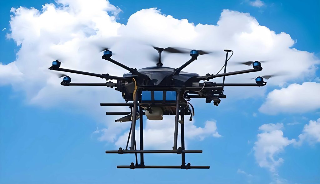
An example of a UAV used in this research is illustrated below.
1. Introduction
Path planning for unmanned aerial vehicles is one of the most active research topics in robotics and autonomous systems. Given a starting point and a target point, the objective is to find a collision-free path that satisfies the kinematic and dynamic constraints of the UAV while optimizing certain criteria such as path length, flight time, energy consumption, and smoothness. In practice, the environment can be known in advance (global static map) or partially unknown with moving obstacles (local dynamic environment). Global path planning algorithms generate a feasible route before the flight, while local path planning algorithms adjust the route in real time based on sensor information. A robust navigation system often combines both approaches to ensure safety and efficiency.
Among global path planning algorithms, graph-search-based methods such as Dijkstra and A* are widely used. They guarantee completeness and optimality under certain heuristics, but their computational complexity grows rapidly with the size of the environment. Sampling-based algorithms such as RRT and probabilistic roadmaps (PRM) are more suitable for high-dimensional and continuous spaces. RRT is particularly popular because it can quickly explore the configuration space by randomly growing a tree from the start to the goal. However, the resulting path is often jagged and far from optimal. Many improvements have been proposed, such as RRT*, informed RRT*, and RRT-Connect. RRT-Connect grows two trees simultaneously, which accelerates the search, but it still inherits the randomness and poor smoothness of RRT.
For local path planning, the artificial potential field (APF) method and the dynamic window approach are widely employed. APF is easy to implement but suffers from local minima and oscillation. DWA performs velocity sampling and trajectory prediction considering the kinematic constraints of the UAV, and it has demonstrated excellent performance in real-time collision avoidance. However, DWA alone cannot guarantee convergence in large complex scenes because it only looks ahead for a short horizon. Therefore, this thesis proposes a fusion framework that uses an improved RRT-Connect as the global planner and an improved DWA as the local planner, with a key-point extraction strategy to guide the local planner along the global path.
2. Theoretical Foundations
2.1 Graph-based Global Path Planning
Dijkstra’s algorithm is a classic single-source shortest-path algorithm. It maintains a set of visited nodes and repeatedly selects the unvisited node with the smallest distance from the start. The distance from the source to each node is updated through relaxation. Dijkstra’s algorithm is guaranteed to find the shortest path in a graph with non-negative edge weights, but its blind search leads to low efficiency. In a 2D grid map, Dijkstra expands almost uniformly from the start to the goal, as observed in many experiments.
A* is an informed version of Dijkstra that uses a heuristic function to guide the search. The evaluation function is given by
$$ f(x) = g(x) + h(x) $$
where $g(x)$ is the cost from the start to node $x$, and $h(x)$ is an admissible heuristic estimating the cost from $x$ to the goal. If $h(x)$ never overestimates the true cost, A* is optimal. In UAV path planning, the Euclidean distance is often used as the heuristic.
2.2 Sampling-based Global Path Planning
2.2.1 RRT Algorithm
The RRT algorithm constructs a tree rooted at the start configuration. In each iteration, a random sample $P_{rand}$ is generated in the free space. The nearest node $P_{near}$ in the tree is found, and a new node $P_{new}$ is created at a fixed distance $\mu$ from $P_{near}$ in the direction of $P_{rand}$. If the edge between $P_{near}$ and $P_{new}$ is collision-free, $P_{new}$ is added to the tree. The process is repeated until the tree connects to the goal region. The pseudocode of the basic RRT algorithm can be summarized as follows:
| Step | Description |
|---|---|
| 1 | Initialize the tree $T$ with the start node $P_s$. |
| 2 | Repeat $N$ times: |
| 3 | Sample a random point $P_{rand}$ from the free space. |
| 4 | Find the nearest node $P_{near}$ in $T$. |
| 5 | Generate $P_{new}$ at distance $\mu$ toward $P_{rand}$. |
| 6 | If the edge is collision-free, add $P_{new}$ to $T$. |
| 7 | If $P_{new}$ is close to the goal, connect and terminate. |
RRT is probabilistically complete, but it does not guarantee optimality. The path quality depends on the sampling distribution and often contains many unnecessary detours.
2.2.2 PRM Algorithm
The probabilistic roadmap (PRM) method consists of a learning phase and a query phase. In the learning phase, random samples are drawn from the configuration space. Samples that lie in the obstacle region are discarded. For each pair of samples whose distance is below a threshold, an edge is created if the connecting segment is collision-free. This builds a graph. In the query phase, the start and goal are connected to the graph, and a graph search algorithm (e.g., A*) is used to find a path. PRM is especially useful for multiple queries in static environments.
2.3 Artificial Potential Field Method
The artificial potential field (APF) method creates an attractive potential around the goal and repulsive potentials around obstacles. The attractive potential function is defined as
$$ U_{att}(P) = \frac{1}{2} \alpha \, D^2(P, P_g) $$
where $\alpha$ is the attractive gain and $D(P, P_g) = \|P – P_g\|$ is the Euclidean distance between the current position $P$ and the goal $P_g$. The attractive force is the negative gradient of the potential:
$$ F_{att}(P) = -\nabla U_{att}(P) = -\alpha (P – P_g) $$
The repulsive potential for obstacle $o$ is defined as
$$ U_{rep}(P) = \begin{cases} \frac{1}{2} \lambda \left( \frac{1}{D(P,P_o)} – \frac{1}{D_0} \right)^2 , & D(P,P_o) \leq D_0 \\ 0, & D(P,P_o) > D_0 \end{cases} $$
where $\lambda$ is the repulsive gain, $P_o$ is the obstacle position, and $D_0$ is the distance of influence. The total force acting on the UAV is the vector sum of the attractive force and the repulsive forces of all obstacles. While APF is simple and reactive, it suffers from local minima and oscillations in cluttered environments.
2.4 UAV Kinematic Constraints
To generate a feasible path, several kinematic constraints must be considered. The minimum flight segment length $L$ defines the shortest distance the UAV must fly before changing direction. The maximum turning angle $\theta_{max}$ limits the heading change between two consecutive segments. Let $\mathbf{s}_1$ and $\mathbf{s}_2$ be the two segment vectors. The turning angle $\theta$ must satisfy
$$ \cos \theta = \frac{\mathbf{s}_1^T \mathbf{s}_2}{\|\mathbf{s}_1\| \|\mathbf{s}_2\|} \geq \cos \theta_{max} $$
The maximum climb/dive angle $\phi_{max}$ in the vertical plane is constrained by
$$ \tan \phi \leq \frac{|z_{new} – z_{near}|}{\sqrt{(x_{new}-x_{near})^2 + (y_{new}-y_{near})^2}} \leq \tan \phi_{max} $$
These constraints are incorporated in the proposed planning algorithms to ensure that the resulting paths are executable by a fixed-wing or multirotor UAV.
2.5 Sensor Model for Obstacle Detection
In dynamic environments, the UAV must detect moving obstacles in real time. A monocular camera is often used for this purpose. The pinhole camera model maps a 3D point $P = [X, Y, Z]^T$ in the camera coordinate system to a 2D pixel coordinate $[u, v]^T$ through
$$ \begin{bmatrix} u \\ v \\ 1 \end{bmatrix} = \frac{1}{Z} K \begin{bmatrix} X \\ Y \\ 1 \end{bmatrix} $$
where $K$ is the intrinsic camera matrix
$$ K = \begin{bmatrix} f_x & 0 & c_x \\ 0 & f_y & c_y \\ 0 & 0 & 1 \end{bmatrix} $$
Here $f_x$ and $f_y$ are the focal lengths in pixels, and $(c_x, c_y)$ is the principal point. To fuse with the world coordinate system, a transformation matrix $T$ is applied, yielding $P_{pixel} = K T P_{world}$. This model enables the UAV to estimate obstacle positions from visual images, which is essential for the local planning module.
3. Global Path Planning Using BGO-RRT
3.1 System Model and Problem Statement
The environment is represented by an occupancy grid map. Let the state space be $\mathcal{P} \subset \mathbb{R}^{n \times n}$ for a 2D square map. The obstacle space is denoted as $\mathcal{P}_{obs}$, and the free space is $\mathcal{P}_{free} = \mathcal{P} \setminus \mathcal{P}_{obs}$. The start and goal positions are $P_s \in \mathcal{P}_{free}$ and $P_g \in \mathcal{P}_{free}$, respectively. A path is a continuous mapping $\sigma: [0,1] \rightarrow \mathcal{P}$ such that $\sigma(0) = P_s$, $\sigma(1) = P_g$, and $\sigma(x) \in \mathcal{P}_{free}$ for all $x \in [0,1]$. The optimal path planning problem is formulated as
$$ \sigma^* = \arg \min_{\sigma \in \Sigma} c(\sigma) $$
where $\Sigma$ is the set of all feasible paths and $c(\sigma)$ is the cost function, typically the Euclidean length of the path.
In this thesis, I also expand the obstacles by one grid cell to account for the physical size of the UAV and to guarantee a safety margin. This inflation is implemented in all simulations.
3.2 The Proposed BGO-RRT Algorithm
The traditional RRT algorithm has three major drawbacks: high randomness, redundant nodes, and poor smoothness. The BGO-RRT algorithm addresses these drawbacks through three effective steps: (1) incorporating an attractive force from the artificial potential field into node generation, (2) applying a greedy pruning algorithm to remove redundant nodes, and (3) using a cubic B-spline curve to smooth the final path.
3.2.1 Attractive Guidance for Node Generation
In each iteration of the growing tree, a random point $P_{rand}$ is generated. Instead of directly expanding toward $P_{rand}$, the new node is also attracted toward the goal. The combined direction is obtained by
$$ P_{new} = P_{near} + \mu \frac{P_{rand} – P_{near}}{\|P_{rand} – P_{near}\|} + \alpha \frac{P_g – P_{near}}{\|P_g – P_{near}\|} $$
where $\mu$ is the extension step size and $\alpha$ is the attractive coefficient. The new node can be computed more explicitly by decomposing the forces. Let $\theta_{rand}$ be the angle of the vector $(P_{rand} – P_{near})$ and $\theta_{goal}$ be the angle of the vector $(P_g – P_{near})$. Then the Cartesian components of the new node are:
$$ \begin{aligned} P_{new,x} &= P_{near,x} + \mu \cos(\theta_{rand}) + \alpha \cos(\theta_{goal}) \\ P_{new,y} &= P_{near,y} + \mu \sin(\theta_{rand}) + \alpha \sin(\theta_{goal}) \end{aligned} $$
After computing the desired position, the node is re-projected to the distance $\mu$ from $P_{near}$ if necessary. This attractive guidance considerably reduces the randomness of the search and focuses the tree growth toward the goal. The comparison between the original RRT and BGO-RRT node searches is summarized in the table below.
| Property | Traditional RRT | BGO-RRT |
|---|---|---|
| Node distribution | Uniformly random | Goal-biased |
| Search efficiency | Low | High |
| Redundant nodes | Many | Fewer |
| Convergence speed | Slow | Fast |
3.2.2 Greedy Pruning Optimization
Even with attractive guidance, the generated path may contain unnecessary intermediate nodes due to the fixed step size. The greedy pruning strategy starts from the goal node $P_g$ and attempts to connect it to the farthest ancestors. For a current node $P_{cur}$, the algorithm checks nodes along the parent chain. If the direct connection from $P_{cur}$ to a candidate node $P_{cand}$ is collision-free, the intermediate nodes are removed and $P_{cand}$ becomes the new predecessor. The process is repeated until the start node is reached. The cost reduction is given by
$$ \Delta L = \sum_{i=1}^{k} \| P_i – P_{i-1} \| – \| P_{cand} – P_{cur} \| $$
where $\| P_i – P_{i-1} \|$ are the original segment lengths. This operation reduces both the path length and the number of turns.
3.2.3 Cubic B-Spline Smoothing
After pruning, the path is a polyline that still has sharp corners. To make it flyable, a cubic B-spline is adopted. Given $n+1$ control points $P_0, P_1, \ldots, P_n$, a cubic B-spline is defined as
$$ C(x) = \sum_{i=0}^{n} P_i B_{i,3}(x) $$
where $B_{i,3}(x)$ are the cubic B-spline basis functions. Using the Cox–de Boor recursion, the basis functions are
$$ B_{i,1}(x) = \begin{cases} 1, & x_i \leq x < x_{i+1} \\ 0, & \text{otherwise} \end{cases} $$
$$ B_{i,k}(x) = \frac{x – x_i}{x_{i+k-1} – x_i} B_{i,k-1}(x) + \frac{x_{i+k} – x}{x_{i+k} – x_{i+1}} B_{i+1,k-1}(x), \quad k \ge 2 $$
For the cubic case, $k=3$. The B-spline curve has $C^2$ continuity, which is sufficient for most UAV autopilots. The control points are chosen as the vertices of the pruned path, and the resulting curve approximates the polyline while reducing curvature variation.
3.3 Pseudocode of BGO-RRT
The complete pseudocode of the BGO-RRT algorithm is presented below.
| Algorithm: BGO-RRT ($P_s$, $P_g$, $M$) |
| 1: Initialize tree $T$ with $P_s$. |
| 2: for $i = 1$ to $M$ do |
| 3: $P_{rand} \leftarrow \text{RANDOM}()$ |
| 4: $P_{near} \leftarrow \text{NEAREST}(P_{rand}, T)$ |
| 5: $P_{att} \leftarrow \text{ATTRACT}(P_{near}, P_g, \alpha)$ |
| 6: if $\text{OBS\_NOT\_FREE}(P_{near}, P_{att})$ then continue |
| 7: $P_{new} \leftarrow \text{NEW\_STATE}(P_{near}, P_{att}, \mu)$ |
| 8: $T.\text{add\_node}(P_{new})$ |
| 9: if $D(P_{new}, P_g) \leq \mu$ and $\text{OBS\_NOT\_FREE}(P_{new}, P_g) = \text{false}$ |
| 10: $T.\text{add\_node}(P_g)$ |
| 11: break |
| 12: end if |
| 13: end for |
| 14: $T \leftarrow \text{PRUNE}(T)$ |
| 15: $T \leftarrow \text{BSPLINE}(T)$ |
| 16: return $T$ |
3.4 Simulation Results of BGO-RRT
I conducted simulations in two representative environments: a narrow-corridor scenario and a complex obstacle scenario. The parameters used in the narrow-corridor scenario are listed below.
| Parameter | Value |
|---|---|
| Map size | 100 × 100 |
| Start point | (10, 15) |
| Goal point | (90, 85) |
| Extension step $\mu$ | 2 |
| Attractive coefficient $\alpha$ | 2 |
The complex obstacle scenario parameters are given in the following table.
| Parameter | Value |
|---|---|
| Map size | 50 × 50 |
| Start point | (0, 0) |
| Goal point | (45, 20) |
| Extension step $\mu$ | 1 |
| Attractive coefficient $\alpha$ | 1 |
For each scenario, I compared the BGO-RRT algorithm with A*, traditional RRT, and ant colony optimization (ACO). The statistical results after 50 independent runs are reported below.
| Scenario | Algorithm | Total Nodes | Planning Time (s) | Failures |
|---|---|---|---|---|
| Narrow corridor | A* | 3776 | 34.51 | 0 |
| RRT | 1014 | 13.49 | 9 | |
| ACO | – | 9.45 | 12 | |
| BGO-RRT | 709 | 6.82 | 0 | |
| Complex obstacle | A* | 702 | 16.19 | 0 |
| RRT | 866 | 9.29 | 2 | |
| ACO | – | 8.32 | 0 | |
| BGO-RRT | 654 | 7.62 | 0 |
The results show that BGO-RRT reduces the number of nodes by about 30% compared with traditional RRT in the narrow corridor scenario and by about 24% in the complex obstacle scenario. The planning time is improved by 49.4% and 18.0% in the two scenarios, respectively. More importantly, the failure rate is reduced to zero, whereas traditional RRT fails in 9 out of 50 runs in the narrow corridor and 2 out of 50 runs in the complex obstacle scenario. The BGO-RRT algorithm also produces a smoother path thanks to B-spline fitting, which is crucial for fixed-wing UAVs that cannot make instantaneous sharp turns.
4. Dynamic Path Planning Based on Fusion of BGO-RRT-Connect and EA-DWA
4.1 System Model and Problem Description
In a real environment, the UAV may encounter moving obstacles whose positions change over time. I model a moving obstacle by its position $(x(t), y(t))$, velocity $v(t)$, and heading direction $\theta(t)$. If the velocity is constant at magnitude $c$, the obstacle motion model is
$$ \begin{aligned} x(t+\Delta t) &= x(t) + c \cos\theta(t) \Delta t \\ y(t+\Delta t) &= y(t) + c \sin\theta(t) \Delta t \end{aligned} $$
The UAV motion is approximated by the following discretized kinematic model:
$$ \begin{aligned} x_{t+1} &= x_t + v \Delta t \cos\theta_t – v \Delta t \sin\theta_t \\ y_{t+1} &= y_t + v \Delta t \sin\theta_t + v \Delta t \cos\theta_t \\ \theta_{t+1} &= \theta_t + w \Delta t \end{aligned} $$
where $v$ is the linear velocity and $w$ is the angular velocity. The dynamic path planning problem is stated as follows: given a global path from the start to the goal, use local sensor information to generate collision-free trajectory segments that keep the UAV as close as possible to the global path while responding to unexpected obstacles.
4.2 Global Path Planning Using BGO-RRT-Connect
RRT-Connect grows two trees: one rooted at the start and the other at the goal. In each iteration, one tree expands toward a random sample, and then the other tree greedily expands toward the newly added node of the first tree. This bidirectional search significantly improves the convergence rate. However, the original RRT-Connect still suffers from high randomness and non-smooth paths. In this thesis, I adopt the same attractive guidance technique used in BGO-RRT to improve node generation for both trees. The new node is generated by
$$ \begin{aligned} P_{new,x} &= P_{near,x} + u \cos \theta + \alpha \cos \theta_g \\ P_{new,y} &= P_{near,y} + u \sin \theta + \alpha \sin \theta_g \end{aligned} $$
where $\theta$ is the direction toward the nearest node of the opposite tree and $\theta_g$ is the direction toward the goal. This strategy accelerates the connection between the two trees while avoiding unnecessary exploration.
The simulation was performed on a 100 m × 100 m map with the start at (0,0), goal at (85,30), step size $u=2$, and attractive coefficient $\alpha=2$. I compared traditional RRT, RRT-Connect, BGO-RRT, and BGO-RRT-Connect. The statistical results after 50 runs are listed in the following table.
| Algorithm | Total Nodes | Path Length (m) | Planning Time (s) | Failures |
|---|---|---|---|---|
| RRT | 796 | 143.8 | 6.65 | 3 |
| RRT-Connect | 316 | 125.3 | 1.64 | 0 |
| BGO-RRT | 242 | 127.9 | 1.35 | 0 |
| BGO-RRT-Connect | 125 | 118.7 | 0.98 | 0 |
The BGO-RRT-Connect algorithm reduces the number of nodes by 84.3% compared with RRT, by 60.4% compared with RRT-Connect, and by 48.4% compared with BGO-RRT. The path length is also decreased by 17.5%, 5.3%, and 7.2%, respectively. The planning time is reduced by 85.3%, 40.2%, and 27.4%, respectively. These improvements demonstrate that BGO-RRT-Connect is an excellent global planner to guide the local planner.
4.3 Dynamic Window Approach and Its Enhancements
4.3.1 Traditional DWA
The dynamic window approach performs local obstacle avoidance by sampling velocities $(v, w)$ from a reduced search space. The search space is the intersection of three sets: the set of admissible velocities considering the maximum and minimum velocities, the set of velocities that allow the UAV to stop before collision, and the set of velocities reachable within one control period considering acceleration constraints. The admissible speed set is
$$ V_a = \{ (v,w) \mid v \in [0, v_{max}], w \in [0, w_{max}] \} $$
The safe speed set is
$$ V_s = \{ (v,w) \mid v \leq \sqrt{2 D(v,w) \dot{v}_b}, w \leq \sqrt{2 D(v,w) \dot{w}_b} \} $$
where $D(v,w)$ is the distance to the nearest obstacle, and $\dot{v}_b$, $\dot{w}_b$ are the linear and angular accelerations. The reachable speed set within time interval $\Delta t$ is
$$ V_d = \{ (v,w) \mid v \in [v_c – \dot{v}_b \Delta t, v_c + \dot{v}_b \Delta t], w \in [w_c – \dot{w}_b \Delta t, w_c + \dot{w}_b \Delta t] \} $$
The final dynamic window is
$$ V_f = V_a \cap V_s \cap V_d $$
For each sampled velocity pair, the trajectory is predicted over a fixed time horizon. The best trajectory is selected by minimizing the cost function
$$ G(v,w) = a_1 \cdot Heading(v,w) + a_2 \cdot Dis(v,w) + a_3 \cdot Vel(v,w) $$
where $Heading(v,w)$ measures the heading alignment with the goal, $Dis(v,w)$ measures the proximity to obstacles, and $Vel(v,w)$ favors higher speeds.
4.3.2 Dual Danger-Range Strategy
Traditional DWA does not explicitly distinguish between obstacles with different levels of threat. To improve the response to fast-moving obstacles, I introduce two danger thresholds: the controllable danger distance $r_1$ and the extreme danger distance $r_2$, with $r_2 < r_1$. Let $d$ be the distance to a moving obstacle. If $d > r_1$, the obstacle is in the safe zone and no action is taken. If $r_2 < d \leq r_1$, the obstacle is in the controllable zone; the UAV reduces its speed to half the current speed and re-evaluates the situation. If $d \leq r_2$, the obstacle is in the extreme danger zone; the UAV immediately stops and replans its local path toward the next waypoint. This simple rule greatly enhances safety in crowded dynamic environments.
4.3.3 Improved Velocity Space
In the conventional DWA, the search space is computed only for the first time interval, which may lose feasible trajectories that require more than one interval to reach. I propose to compute the achievable velocity space over the entire prediction horizon. The improved velocity space is
$$ V_p = \left\{ (v,w) \middle| \begin{array}{l} v \in [\max(0, v_0 – \dot{v}_{b,max} T), \min(v_{\max}, v_0 + \dot{v}_{b,max} T)] \\ w \in [\max(w_{\min}, w_0 – \dot{w}_{b,max} T), \min(w_{\max}, w_0 + \dot{w}_{b,max} T)] \end{array} \right\} $$
where $T$ is the prediction horizon, $v_0$ and $w_0$ are the current velocities, and $\dot{v}_{b,max}$, $\dot{w}_{b,max}$ are the maximum accelerations. This expansion allows the DWA to consider more diverse trajectories and improves its predictive ability.
4.3.4 Improved Evaluation Function
The original evaluation function lacks a smoothness term. I add an angular-change term $Ang(v,w)$ defined as
$$ Ang(v,w) = \left| \theta_{goal} – \theta_i \right| – \left| \theta_{start} – \theta_i \right| $$
or equivalently
$$ Ang(v,w) = 180^\circ – | \theta_{gi} – \theta_{si} | $$
where $\theta_{gi}$ is the heading at the end of the predicted trajectory and $\theta_{si}$ is the initial heading of the UAV. After normalization, the enhanced evaluation function is
$$ G_{EA}(v,w) = a_1 \cdot Heading(v,w) + a_2 \cdot Dis(v,w) + a_3 \cdot Vel(v,w) + a_4 \cdot Ang(v,w) $$
where $a_4$ is the weight for the angular-change term. This term penalizes trajectories that change direction too frequently, leading to smoother paths and reduced energy consumption.
4.4 Fusion Strategy
The fusion of BGO-RRT-Connect and EA-DWA is achieved by extracting waypoints from the global path and using them as sub-goals for the local planner. The extraction process filters out collinear and redundant nodes. Given a set of path nodes $\{P_0, P_1, \ldots, P_n\}$, I compute the angle between consecutive segments. If the angle is near zero, the middle node is removed. For non-collinear nodes, the algorithm checks the distance from the line segment connecting $P_i$ and $P_{i+2}$ to obstacles. If the distance is larger than a safety threshold, $P_{i+1}$ is removed; otherwise, $P_{i+2}$ is kept as a key point. The resulting key-point set is then fed to the EA-DWA local planner one by one. The flow of the fusion algorithm is as follows:
| 1. Use BGO-RRT-Connect to generate the global path $\mathcal{G}$. |
| 2. Extract key points $\mathcal{K} = \{K_1, K_2, \ldots, K_m\}$ from $\mathcal{G}$. |
| 3. Set the first key point as the current sub-goal. |
| 4. While the UAV has not reached the final goal: |
| 5. Detect obstacles using sensors. |
| 6. Apply the EA-DWA algorithm to compute the optimal velocity. |
| 7. Execute the motion for one control period. |
| 8. If the current sub-goal is reached, switch to the next key point. |
| 9. End while. |
This method guarantees that the local planner always has a feasible global reference, thus avoiding the local minimum problem of pure DWA.
4.5 Simulation Results of EA-DWA
I first evaluated EA-DWA in a 10 m × 10 m map with four moving obstacles. The UAV starts at (0,0) and aims at (10,8). The dynamic obstacles move back and forth along predefined segments. The parameters are listed below.
| Parameter | Value |
|---|---|
| UAV max linear velocity | 2 m/s |
| UAV max angular velocity | $\pi/9$ rad/s |
| Linear acceleration | 0.2 m/s² |
| Angular acceleration | $5\pi/18$ rad/s² |
| $a_1$ | 0.05 |
| $a_2$ | 0.05 |
| $a_3$ | 0.35 |
| $a_4$ | 0.15 |
| $r_1$ | 3 m |
| $r_2$ | 2 m |
I compared EA-DWA with traditional DWA. The results over 10 runs are shown in the following table.
| Algorithm | Path Length (m) | Planning Time (s) | Total Turning Angle (°) | Collisions |
|---|---|---|---|---|
| DWA | 14.55 | 54.7 | 95 | 4 |
| EA-DWA | 13.64 | 43.2 | 68 | 0 |
EA-DWA reduces the average path length by 6.25%, the planning time by 21.03%, and the total turning angle by 28.42%. In addition, traditional DWA experienced four collision failures, while EA-DWA did not fail in any of the ten runs. This demonstrates that the dual danger-range strategy and the improved evaluation function contribute to safer and more efficient dynamic obstacle avoidance.
4.6 Simulation Results of the Fusion Algorithm
Finally, I tested the complete fusion system in a larger environment of size 100 m × 100 m. The start is at (0,0), and the goal is at (50,90). Two dynamic obstacles of size 5 m × 5 m move back and forth along segments centered at (27.5,22.5)–(27.5,12.5) and (57.5,72.5)–(67.5,72.5), respectively, with a speed of 2 m/s. The UAV maximum linear velocity is 6 m/s, and the maximum angular velocity is $\pi/4$ rad/s. The parameters of the EA-DWA are $a_1=0.05$, $a_2=0.05$, $a_3=0.35$, $a_4=0.15$, $r_1=5$ m, and $r_2=2$ m.
I compared three baselines: (a) the fusion of BGO-RRT-Connect with traditional DWA, (b) the algorithm from a representative reference that combines artificial potential field with RRT, and (c) an A*-DWA hybrid algorithm from another reference. The results without dynamic obstacles are shown in the table below.
| Algorithm | Planning Time (s) | Path Length (m) | Total Turning Angle (°) |
|---|---|---|---|
| BGO-RRT-Connect + DWA | 187.2 | 142.5 | 426.5 |
| Reference [57] | 174.3 | 132.9 | 497.2 |
| Reference [58] | 186.1 | 124.7 | 161.5 |
| BGO-RRT-Connect + EA-DWA (proposed) | 172.7 | 128.4 | 103.6 |
The proposed fusion algorithm achieves the shortest planning time of 172.7 s and the smallest total turning angle of 103.6°, which indicates a much smoother trajectory. Although the path length is slightly longer than reference [58] by 2.97%, the reduction in turning angle and planning time compensates for this small difference.
When dynamic obstacles are added, the results are summarized in the following table.
| Algorithm | Planning Time (s) | Path Length (m) | Total Turning Angle (°) | Failures |
|---|---|---|---|---|
| BGO-RRT-Connect + DWA | 196.5 | 168.3 | 483.4 | 3 |
| Reference [57] | 185.7 | 147.7 | 455.2 | 0 |
| Reference [58] | 194.5 | 143.5 | 257.0 | 1 |
| BGO-RRT-Connect + EA-DWA (proposed) | 178.1 | 140.7 | 253.0 | 0 |
The proposed algorithm outperforms all baselines in terms of planning time, path length, total turning angle, and failure count. It reduces the planning time by 9.36% compared with BGO-RRT-Connect + DWA, by 4.1% compared with reference [57], and by 8.43% compared with reference [58]. The total turning angle is reduced by 46.93%, 4.44%, and 1.56% relative to the three baselines, respectively. Moreover, the proposed algorithm did not fail in any of the ten runs, while the traditional DWA fusion failed three times and reference [58] failed once. This confirms that the dual danger-range strategy and the improved evaluation function significantly enhance robustness in dynamic environments.
5. Conclusion and Future Work
In this thesis, I have studied the path planning problem for unmanned aerial vehicles in both static and dynamic environments. The main contributions are as follows.
First, I proposed the BGO-RRT algorithm for global path planning. The algorithm integrates an attractive force into the RRT node expansion, which greatly reduces the randomness of the search. A greedy pruning procedure removes redundant nodes and shortens the path. A cubic B-spline curve is then used to smooth the resulting polyline, making it suitable for fixed-wing UAVs. Simulations in narrow-corridor and complex-obstacle scenarios show that BGO-RRT significantly improves planning efficiency and success rate compared with A*, RRT, and ant colony optimization.
Second, I proposed the BGO-RRT-Connect algorithm, which extends the same attractive guidance to the bidirectional search of RRT-Connect. This algorithm produces a high-quality global path with fewer nodes and shorter length, making it ideal for guiding local planners.
Third, I developed the EA-DWA algorithm for local dynamic obstacle avoidance. The improvements include a dual danger-range strategy, an expanded velocity space, and a new angular-change evaluation term. These enhancements enable the UAV to react to fast-moving obstacles and to produce smoother local trajectories. The fusion of BGO-RRT-Connect and EA-DWA combines the strengths of global and local planning. The global path provides a sequence of key points, and the local planner uses the enhanced DWA to move between these points while avoiding unexpected obstacles. Extensive simulations demonstrate that the fusion algorithm achieves shorter planning time, shorter path length, smaller turning angle, and zero failures in dynamic environments.
Despite these encouraging results, there are several limitations. The simulations are currently performed in a two-dimensional grid map. Real unmanned aerial vehicles operate in three-dimensional space, so extending the proposed algorithms to 3D environments is a natural next step. In 3D, the state space includes altitude, and the dynamic constraints become more complex. I plan to address this by incorporating a 3D occupancy map and adapting the sampling and velocity space accordingly.
Another limitation is that the algorithms have not been tested on physical UAV platforms. To validate the practical applicability, I intend to integrate the proposed planners with a flight controller and conduct field experiments. Real-world issues such as sensor noise, communication delays, and wind disturbances must be considered. Robustness analysis and hardware-in-the-loop simulations will be part of future work.
Furthermore, the current B-spline smoothing is performed off-line after the global path is generated. In dynamic scenarios, the local path may deviate from the global spline. An online trajectory re-planning mechanism using B-splines or minimum-snap polynomials could further improve flight performance. This would allow the UAV to regenerate smooth and dynamically feasible trajectories in real time.
Finally, the weights in the improved DWA evaluation function are manually tuned. Future studies can employ adaptive or learning-based methods, such as fuzzy logic or reinforcement learning, to adjust these weights online based on the environment and mission requirements. This would make the path planning system more flexible and intelligent.
In summary, this thesis provides effective solutions for both global and local path planning of unmanned aerial vehicles. The proposed algorithms show significant improvements over traditional methods in simulation. With further refinement and experimental validation, these methods have the potential to enhance the autonomy and safety of UAV operations in complex real-world environments.