
In recent years, the rapid advancement of unmanned aerial vehicles (UAVs) has enabled their widespread deployment in fields such as environmental monitoring, infrastructure inspection, precision agriculture, and emergency response. As a core perception technology for these applications, object detection in UAV aerial images has attracted increasing attention. However, compared with ordinary images, aerial images captured by unmanned aerial vehicles exhibit several unique challenges: targets are often extremely small, densely packed, heavily occluded, and subject to significant scale variations due to changing flight altitude and viewing angle. Additionally, complex backgrounds and varying illumination conditions further increase the difficulty of accurate detection. Traditional detection algorithms rely on hand-crafted features and sliding-window search strategies, which are both computationally expensive and insufficiently expressive for such challenging scenarios. Deep learning-based detectors, especially the YOLO family, have greatly improved the accuracy and speed of object detection, but they still face serious performance degradation when applied to small objects in UAV imagery. Moreover, onboard UAV platforms have limited computational resources and strict power budgets, making it difficult to deploy large-scale models with high complexity. Therefore, designing a detection algorithm that simultaneously achieves high accuracy and high efficiency for small object detection in unmanned aerial vehicles remains a significant research problem.
In this paper, I present a systematic investigation into improving the YOLOv11 baseline for UAV aerial image object detection. My work is organized into two main parts. First, I propose an enhanced detection model, termed EGD-YOLO, which incorporates three novel components: a dual-path convolution efficient layer aggregation network (ELAN-DC), a global-to-local bidirectional feature pyramid network (GLBiFPN), and a dynamic detection head (DyHead). These components are designed to improve feature extraction, multi-scale feature fusion, and adaptive feature refinement, respectively. Second, to address the deployment constraints of unmanned aerial vehicles, I further propose a lightweight model EGD-YOLO-Lite based on the BiFPN feature fusion structure, LAMP structured pruning, and CWD channel-wise feature distillation. The proposed lightweight model significantly reduces the parameter count and computational cost while maintaining competitive detection accuracy. Extensive experiments on the VisDrone2019 and DOTA datasets demonstrate the effectiveness and superiority of the proposed methods.
1. Introduction
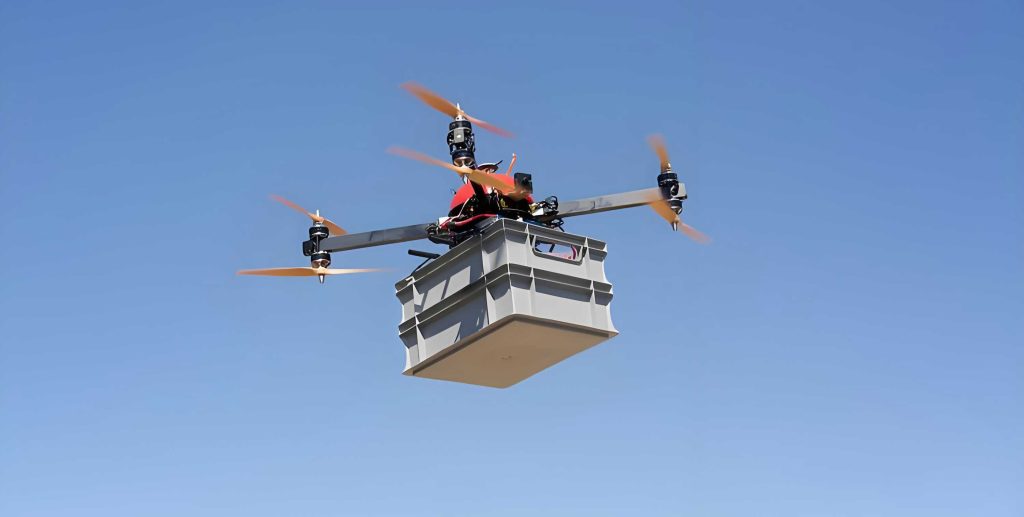
Object detection in images captured by unmanned aerial vehicles plays a vital role in numerous practical applications. For instance, in intelligent transportation systems, UAV-based detectors can automatically identify vehicles, pedestrians, and traffic violations, providing valuable data for traffic flow analysis and city planning. In ecological monitoring, they help locate rare animals and detect illegal activities such as poaching. During disaster response, UAVs search for trapped people and assess structural damage, dramatically improving rescue efficiency. In military surveillance, real-time target detection from aerial platforms enhances situational awareness and operational effectiveness. A representative illustration of typical UAV application scenarios is shown in the figure above.
Despite the great potential of UAV-based object detection, several critical challenges remain. The most prominent issue is the small target size. Objects in aerial images often occupy only a few pixels, providing insufficient appearance information for robust recognition. Furthermore, due to the high altitude of unmanned aerial vehicles, targets exhibit large scale variations. For example, a car may appear as a tiny blob in one frame and become a relatively large object in another frame when the UAV descends. This scale diversity makes fixed-size receptive fields inadequate. In addition, complex backgrounds with dense textures, shadows, and similar-looking non-target regions can easily distract the detector, leading to false positives. Weather conditions, such as haze, rain, and low illumination, further degrade image quality and obscure target boundaries.
To overcome these challenges, the research community has devoted significant efforts to developing robust and efficient detection algorithms. Early traditional methods, such as HOG-based detectors and DPM, used hand-crafted features and were too slow and fragile for real-world UAV applications. With the advent of deep learning, two-stage detectors like R-CNN, Fast R-CNN, and Faster R-CNN achieved high accuracy by generating region proposals and then classifying each proposal. However, their heavy computational burden made them unsuitable for real-time UAV deployment. One-stage detectors, especially the YOLO series, offer a favorable trade-off between speed and accuracy. Starting from YOLOv1, the YOLO family has evolved through multiple generations, introducing improvements such as multi-scale detection, feature pyramid networks, CSPNet-based backbones, anchor-free mechanisms, and efficient attention modules. YOLOv11, the latest iteration, presents a well-designed backbone with C3k2 and C2PSA modules, a PAN-FPN neck, and a lightweight detection head using depthwise convolutions. Although YOLOv11 achieves impressive results on general object detection benchmarks, its performance on small objects in UAV imagery is still suboptimal. Therefore, I choose YOLOv11 as the baseline and make targeted modifications to better adapt it to the UAV domain.
2. Related Work
2.1 Traditional object detection
Traditional object detection methods usually consist of three stages: candidate region generation, hand-crafted feature extraction, and classification. Sliding windows are used to scan the input image at multiple scales to propose candidate regions. Then, features such as HOG or SIFT are extracted from each region. Finally, classifiers such as AdaBoost or SVM are applied to determine whether the region contains an object of interest. Non-maximum suppression is typically employed to remove duplicate boxes. These methods are computationally inefficient because they evaluate a large number of windows, and their feature representations lack the semantic richness needed for complex scenes.
2.2 Deep learning based object detection
Deep learning based detectors can be divided into two-stage and one-stage families. Two-stage detectors, represented by R-CNN and its successors, first generate region proposals through a separate module (e.g., RPN) and then perform classification and regression on these proposals. They generally achieve higher accuracy but at the expense of speed. One-stage detectors, such as YOLO and SSD, directly predict objects from the input image in a single forward pass. They are much faster, which makes them ideal for real-time applications on drones. Recent YOLO versions have introduced more efficient backbone structures, advanced feature fusion methods, and better training strategies, gradually narrowing the accuracy gap with two-stage detectors. YOLOv11 is particularly notable for its strong performance and flexible design.
2.3 Small object detection in UAV images
To handle small objects in UAV aerial images, researchers have proposed various improvements. Some works introduce specialized feature extraction modules, such as deformable convolutions, multi-branch dilated convolutions, and attention mechanisms. Others focus on enhancing the neck network through richer feature pyramid structures, like cross-scale feature fusion and repeated top-down/bottom-up pathways. Some add an extra P2 layer to preserve high-resolution features for small objects. Additionally, there are attempts to design better loss functions that emphasize small objects or to adopt multi-scale training strategies. However, many of these methods increase the model size and computational workload, making them unsuitable for embedded UAV platforms. Therefore, achieving a good balance between detection performance and model efficiency remains a key research direction.
3. Proposed EGD-YOLO
3.1 Overall architecture
I propose the EGD-YOLO model based on YOLOv11 with three major modifications. The overall architecture is depicted conceptually as follows: the backbone uses ELAN-DC blocks to replace the original C3k2 blocks; the neck is reconstructed into GLBiFPN which incorporates GLSA modules into a bidirectional feature pyramid network; the original detection head is replaced by DyHead. This design aims to boost the feature representation capability for small objects while enhancing multi-scale information interaction and adaptive feature selection.
3.2 Dual-Conv Efficient Layer Aggregation Network (ELAN-DC)
To strengthen feature extraction without incurring excessive computational cost, I design ELAN-DC by integrating the Dual-Conv (DC) unit into the ELAN architecture. The Dual-Conv module combines a 3×3 convolution and a 1×1 convolution in a dual-pathway layout. The 3×3 convolution captures richer spatial details and enlarges the receptive field, which is crucial for detecting small objects whose pixel occupancy is low. The 1×1 convolution performs cross-channel feature aggregation and reduces the feature dimensionality, thereby decreasing computation. The structure of Dual-Conv can be described mathematically. Let $X$ denote the input feature map. The two branches produce outputs:
$$ Y_{3}=f_{3\times3}(X), \quad Y_{1}=f_{1\times1}(X) $$
where $f_{3\times3}$ and $f_{1\times1}$ denote convolutional layers with kernel sizes 3×3 and 1×1, respectively. The output of the Dual-Conv module is then obtained by concatenating the two branch outputs along the channel dimension and passing them through a final 1×1 convolution:
$$ Y_{out} = f_{1\times1}^{proj}([Y_{3}, Y_{1}]) $$
In the ELAN-DC block, the input feature is first split into two branches along the channel dimension. One branch is kept as an identity mapping, while the other is processed by a cascade of Dual-Conv modules. At the end, both branches are concatenated and fused by a 1×1 convolution. This design promotes feature reuse, preserves fine-grained details, and reduces parameter redundancy. The ELAN-DC block can be expressed as:
$$ F_{out} = H_{1\times1}(\; [F_{id}, \; G_{3}(…) G_{1}(…) ] \;) $$
where $H_{1\times1}$ is the fusion convolution, $F_{id}$ is the identity branch, and $G_i$ denotes the i-th Dual-Conv module.
3.3 Global-to-Local Bidirectional Feature Pyramid Network (GLBiFPN)
The default YOLOv11 neck uses a PAN-FPN structure that combines top-down and bottom-up pathways. However, this simple fusion strategy often loses important small-object information when features undergo multiple downsampling operations. I propose GLBiFPN which enhances the BiFPN architecture with Global-to-Local Spatial Attention (GLSA) blocks. BiFPN introduces weighted feature fusion to combine features from different scales with learnable weights. For a node at level $i$, its output is computed as:
$$ P_i^{out} = \sigma \left( \sum_{j} w_{ij} \cdot \text{Resize}(P_j^{in}) \right) $$
where $w_{ij}$ are learnable weights normalized by softmax, and Resize denotes upsampling or downsampling operations. To further refine the fused features, I insert GLSA blocks into selected fusion nodes. GLSA splits the input feature $F_i$ into two channel-wise halves: $F_i^1$ and $F_i^2$. The first half goes through global spatial attention (GSA) which computes global dependencies across spatial positions using a self-attention mechanism. The second half goes through local spatial attention (LSA) which applies depthwise convolution to capture local contextual details. The formal definitions are given by:
$$ F_i^1, F_i^2 = \text{Split}(F_i) $$
$$ F_i’ = f_{1\times1}^{cat}(\; [\text{GSA}(F_i^1), \; \text{LSA}(F_i^2)] \;) $$
The GSA operation can be formulated as:
$$ \text{GSA}(F^1) = \text{MLP}(\; \text{Softmax}(F^1 \cdot (F^1)^T ) \cdot F^1 \;) $$
while the LSA operation uses a bottleneck with depthwise 3×3 convolution:
$$ \text{LSA}(F^2) = f_{1\times1}(\; \sigma(f_{1\times1}^{reduce}(DWConv_{3\times3}(F^2))) \;) \odot F^2 $$
where $\sigma$ is the sigmoid function, $\odot$ denotes element-wise multiplication, and $DWConv$ is depthwise convolution. This hybrid attention module effectively combines global context and local details, allowing the neck to maintain high-resolution small-object features while leveraging semantic information from deeper layers.
3.4 Dynamic Head (DyHead)
The standard detection head of YOLOv11 uses separate branches for classification and regression with fixed convolutional kernels. This limits the model’s ability to adaptively focus on important features, especially in complex UAV scenes with severe scale variation. I adopt the Dynamic Head (DyHead) which unifies scale awareness, spatial awareness, and task awareness through attention mechanisms. DyHead applies three sequential attention operations on the feature tensor $F$ of shape $L \times S \times C$, where $L$ is the number of pyramid levels, $S$ is the spatial dimension, and $C$ is the channel dimension:
$$ W(F) = \pi_C( \pi_S( \pi_L(F) \cdot F ) \cdot F ) \cdot F $$
Here, $\pi_L$ is the scale-aware attention that dynamically adjusts weights across scales, $\pi_S$ is the spatial-aware attention that focuses on critical spatial regions, and $\pi_C$ is the task-aware attention that adaptively selects feature channels for different tasks (classification and regression). These attentions are implemented using lightweight fully connected layers and activation functions. By replacing the original head with DyHead, the model can better adapt to targets of extreme scales and complex backgrounds, thus reducing false positives and missed detections.
4. Experimental Evaluation of EGD-YOLO
4.1 Datasets and settings
I evaluate EGD-YOLO primarily on the VisDrone2019 dataset, which contains 6,471 training images, 548 validation images, and 1,610 test images. The dataset comprises 10 categories: pedestrian, people, bicycle, car, van, truck, tricycle, awning-tricycle, bus, and motor. All images are captured from drones in various urban and suburban scenes with complex backgrounds. I also use the DOTAv1.0 dataset for cross-dataset validation. For training, all images are resized to 640×640. The batch size is set to 8 and the optimizer is SGD with momentum. The models are trained for 200 epochs in most experiments. The hardware environment includes an Intel i5-12400F CPU and an NVIDIA RTX 4060-TI GPU (16GB).
4.2 Evaluation metrics
To comprehensively evaluate model performance, I use the following metrics:
- Precision (P): $P = \frac{TP}{TP+FP}$
- Recall (R): $R = \frac{TP}{TP+FN}$
- Mean Average Precision (mAP): $mAP = \frac{1}{N}\sum_{i=1}^{N} AP_i$
- $mAP@50$ and $mAP@50\text{-}95$ with varying IoU thresholds
- Parameters (Param) and GFLOPs for model complexity
4.3 Ablation studies on VisDrone2019
To verify the contribution of each proposed module, I conduct a series of ablation experiments. The baseline is YOLOv11n. The three enhancement modules are denoted as A = ELAN-DC, B = GLBiFPN, and C = DyHead. Results are shown in the following table.
| Model | P (%) | R (%) | mAP@50 (%) | mAP@50-95 (%) | Param (M) | GFLOPs |
|---|---|---|---|---|---|---|
| Baseline | 43.8 | 33.3 | 33.3 | 19.4 | 2.58 | 6.3 |
| Baseline + A | 43.5 | 34.1 | 33.8 | 19.6 | 2.43 | 6.9 |
| Baseline + B | 44.2 | 34.0 | 34.0 | 20.2 | 2.07 | 6.7 |
| Baseline + C | 46.7 | 35.1 | 35.7 | 21.1 | 3.10 | 7.5 |
| Baseline + A + B | 46.1 | 35.6 | 36.2 | 21.3 | 2.46 | 9.7 |
| Baseline + A + C | 47.8 | 35.8 | 36.7 | 21.7 | 2.95 | 8.0 |
| Baseline + B + C | 47.1 | 36.0 | 36.0 | 21.4 | 2.70 | 8.0 |
| Baseline + A + B + C (EGD-YOLO) | 47.7 | 37.7 | 38.4 | 22.9 | 3.01 | 10.5 |
From Table 1, each module contributes positively to the final performance. Specifically, the ELAN-DC module improves mAP@50 by 0.5% and mAP@50-95 by 0.2% over the baseline while slightly reducing parameters. The GLBiFPN module brings gains of 0.7% in mAP@50 and 0.8% in mAP@50-95. The most significant boost comes from DyHead, which increases mAP@50 by 2.4% and mAP@50-95 by 1.7%. When all three modules are integrated, the final EGD-YOLO achieves mAP@50 of 38.4% and mAP@50-95 of 22.9%, which are 5.1% and 3.5% higher than the baseline, respectively. Although the total model complexity increases, it is still much lower than YOLOv11s: EGD-YOLO has 3.01M parameters versus 9.41M for YOLOv11s, and 10.5 GFLOPs versus 21.3 GFLOPs.
4.4 Comparison with state-of-the-art methods
I compare EGD-YOLO with several mainstream detectors on VisDrone2019. The results are summarized in Table 2.
| Model | Param (M) | GFLOPs | P (%) | R (%) | mAP@50 (%) | mAP@50-95 (%) |
|---|---|---|---|---|---|---|
| Faster R-CNN | 41.0 | 207.0 | 45.5 | 32.2 | 33.1 | 16.0 |
| YOLOv5s | 9.1 | 24.1 | 50.0 | 38.5 | 33.9 | 23.2 |
| YOLOv7tiny | 6.01 | 13.1 | 50.3 | 37.6 | 32.7 | 16.0 |
| YOLOv8n | 3.0 | 8.1 | 45.4 | 32.6 | 33.1 | 19.4 |
| YOLOv10s | 8.04 | 24.5 | 50.5 | 38.3 | 39.1 | 23.5 |
| YOLOv11n | 2.58 | 6.3 | 43.8 | 33.3 | 33.3 | 19.4 |
| YOLOv11s | 9.41 | 21.3 | 50.5 | 38.7 | 39.3 | 23.6 |
| EGD-YOLO (Ours) | 3.01 | 10.5 | 47.7 | 37.7 | 38.4 | 22.9 |
It can be observed that EGD-YOLO outperforms the baseline YOLOv11n by a large margin, with improvements of 5.1% in mAP@50 and 3.5% in mAP@50-95. Compared with YOLOv8n, the proposed model improves mAP@50 by 5.3% and mAP@50-95 by 3.5%. Although EGD-YOLO does not surpass YOLOv11s in raw mAP, its number of parameters is only about one-third of YOLOv11s, and its GFLOPs is less than half. This demonstrates that EGD-YOLO achieves a favorable balance between accuracy and efficiency, making it more suitable for resource-constrained unmanned aerial vehicles.
4.5 Cross-dataset validation
To assess generalization capability, I also conduct experiments on DOTAv1.5 and COCO datasets. The obtained results are presented in Table 3.
| Dataset | Model | P (%) | R (%) | mAP@50 (%) | mAP@50-95 (%) |
|---|---|---|---|---|---|
| DOTAv1.5 | YOLOv11n | 69.2 | 32.3 | 36.2 | 21.7 |
| DOTAv1.5 | EGD-YOLO | 73.4 | 33.5 | 37.7 | 23.0 |
| COCO | YOLOv11n | 61.4 | 44.8 | 49.0 | 34.4 |
| COCO | EGD-YOLO | 61.6 | 46.5 | 50.3 | 35.3 |
| VisDrone2019 | YOLOv11n | 43.8 | 33.3 | 33.3 | 19.4 |
| VisDrone2019 | EGD-YOLO | 47.7 | 37.7 | 38.4 | 22.9 |
The results indicate that EGD-YOLO consistently improves detection accuracy across multiple datasets, demonstrating good generalization and robustness. The improvements are particularly notable in the UAV-focused VisDrone2019 dataset, confirming the effectiveness of the proposed enhancements for small object detection in unmanned aerial vehicles.
5. Lightweight Model: EGD-YOLO-Lite
5.1 Motivation
Although EGD-YOLO achieves high detection accuracy, its increased computational complexity may hinder deployment on embedded UAV platforms. In many real-world applications, the onboard computer of a UAV has limited GPU capability and memory. Therefore, I further propose EGD-YOLO-Lite, a lightweight variant that reduces parameters and computational overhead while preserving as much accuracy as possible. The lightweight design comprises three steps: (1) replacing the heavy feature fusion neck with the more efficient BiFPN; (2) applying LAMP structured pruning to remove redundant channels; and (3) using CWD channel-wise feature distillation to recover performance loss caused by pruning.
5.2 BiFPN feature fusion network
BiFPN provides a more compact multi-scale feature fusion approach than PAFPN. It removes nodes with only one input edge and introduces bidirectional cross-scale connections. Each fused feature is computed using learnable weights:
$$ O_i = \text{Conv}\left( \frac{w_1 \cdot \text{Up}(P_{i+1}) + w_2 \cdot P_i}{w_1 + w_2 + \epsilon} \right) $$
BiFPN effectively reduces the number of parameters while preserving multi-scale representation capability. In my experiments, using BiFPN alone reduces the parameter count from 3.01M to 2.86M and GFLOPs from 10.5 to 10.0 with only a slight drop of 0.2% in mAP@50.
5.3 LAMP structured pruning
To further compress the model, I adopt the Layer-Adaptive Magnitude-based Pruning (LAMP) method. LAMP assigns a score to each weight based on its magnitude and layer context. For a flattened weight vector $W^{(l)}$ of layer $l$, the LAMP score of the $u$-th element is:
$$ \text{Score}(u; W^{(l)}) = \frac{(W^{(l)}[u])^2}{\sum_{v \geq u} (W^{(l)}[v])^2} $$
where the weights are sorted by their absolute magnitude in ascending order. The numerator represents the squared magnitude of the current weight, and the denominator is the sum of squared magnitudes of all weights with larger or equal values in the same layer. This score measures the relative contribution of each weight to the layer’s output. We then prune the connections with the lowest scores according to a global or local compression ratio. In my experiments, I found that local pruning, where each layer is pruned independently according to its ratio, yields better performance than global pruning. I also compared different pruning ratios to find the optimal trade-off. The results are shown in Table 4.
| Speedup | mAP@50 (%) | mAP@50-95 (%) | Param (M) | GFLOPs |
|---|---|---|---|---|
| 1.0 (no pruning) | 38.2 | 23.0 | 2.86 | 10.0 |
| 1.5 | 37.4 | 21.8 | 1.94 | 6.6 |
| 1.6 | 36.6 | 21.3 | 1.84 | 6.2 |
| 1.7 | 35.6 | 20.9 | 1.75 | 5.8 |
| 1.8 | 34.9 | 20.4 | 1.65 | 5.5 |
| 2.0 | 33.1 | 19.2 | 1.52 | 5.0 |
I observe that a speedup of 1.5× provides a good balance: the parameter count drops by about 32%, and GFLOPs reduce by 34%, while mAP@50 only decreases by 0.8 percentage points. Higher compression ratios lead to more significant performance degradation. Therefore, I select the 1.5× pruned model as the student model for subsequent distillation.
5.4 CWD feature distillation
To compensate for the accuracy loss introduced by pruning, I employ Channel-Wise knowledge Distillation (CWD). Unlike traditional distillation based on logits, CWD aligns the channel-wise probability distributions of the teacher and student models. For each channel $c$, the feature map is normalized through a softmax operation across spatial positions:
$$ \varphi(y_c) = \frac{e^{y_{c,i}/\tau}}{\sum_{i} e^{y_{c,i}/\tau}} $$
where $\tau$ is a temperature hyperparameter. The distillation loss is the KL divergence between the teacher and student probability maps, averaged over all channels:
$$ L_{CWD} = \frac{1}{C} \sum_{c=1}^{C} \sum_{i} \varphi(y_{c,i}^T) \log \frac{\varphi(y_{c,i}^T)}{\varphi(y_{c,i}^S)} $$
By minimizing this loss, the student model learns to produce similar activation patterns to the teacher, preserving important spatial information that is crucial for small object detection.
5.5 Overall lightweight pipeline
In my implementation, I first train an unpruned EGD-YOLO-Lite-s model with a larger depth and width scale to serve as the teacher. The teacher model achieves higher mAP@50 (41.5%) than both YOLOv11s and the unpruned n-size model. The student model is the 1.5× LAMP-pruned version of EGD-YOLO-Lite-n. After pruning, the model is fine-tuned on VisDrone2019. Then CWD distillation is applied using the teacher model to guide the student. The complete ablation results for EGD-YOLO-Lite are shown in Table 5.
| Baseline | BiFPN | LAMP | CWD | mAP@50 (%) | Weight (MB) | Param (M) | GFLOPs |
|---|---|---|---|---|---|---|---|
| √ | 38.4 | 6.1 | 3.01 | 10.5 | |||
| √ | √ | 38.2 | 5.8 | 2.86 | 10.0 | ||
| √ | √ | √ | 37.4 | 4.0 | 1.94 | 6.6 | |
| √ | √ | √ | √ | 37.6 | 4.0 | 1.94 | 6.6 |
From Table 5, BiFPN reduces model size slightly, LAMP pruning introduces a 0.8% drop in mAP@50, and CWD distillation recovers 0.2% of performance while keeping the model size unchanged. Compared with the original EGD-YOLO, the final EGD-YOLO-Lite retains a mAP@50 of 37.6% (a loss of only 0.8%) while reducing parameters from 3.01M to 1.94M (a reduction of about 36%) and GFLOPs from 10.5 to 6.6 (a reduction of about 37%).
5.6 Comparison of lightweight models
I further compare EGD-YOLO-Lite with several lightweight detectors, as listed in Table 6.
| Model | Param (M) | GFLOPs | mAP@50 (%) | mAP@50-95 (%) |
|---|---|---|---|---|
| YOLOv5s | 9.1 | 24.1 | 33.9 | 23.2 |
| YOLOv7tiny | 6.01 | 13.1 | 32.7 | 16.0 |
| YOLOv8n | 3.0 | 8.1 | 33.1 | 19.4 |
| AFL-YOLOv8 | 2.38 | 15.9 | 32.8 | 19.5 |
| WCCE-YOLO | – | – | 37.3 | 21.6 |
| YOLOv11n | 2.58 | 6.3 | 33.3 | 19.4 |
| EGD-YOLO | 3.01 | 10.5 | 38.4 | 22.9 |
| EGD-YOLO-Lite (Ours) | 1.94 | 6.6 | 37.6 | 22.1 |
The final lightweight model achieves the highest mAP@50 among all compact models, with only 1.94M parameters and 6.6 GFLOPs. It even outperforms YOLOv11n by 4.3% in mAP@50 while having 24.8% fewer parameters and roughly the same computational cost. This demonstrates the effectiveness of the proposed combination of BiFPN, LAMP pruning, and CWD distillation for creating efficient UAV-deployable detectors.
5.7 Pruning method comparison and teacher selection
I also compared LAMP with a state-of-the-art pruning method, Group-Taylor, under the same target computation budget. The results are shown in Table 7.
| Method | P (%) | R (%) | mAP@50 (%) | Weight (MB) | GFLOPs |
|---|---|---|---|---|---|
| No pruning | 50.6 | 36.7 | 38.2 | 5.8 | 10.0 |
| Group-Taylor | 39.2 | 25.6 | 25.8 | 3.1 | 5.0 |
| LAMP | 44.4 | 32.7 | 33.1 | 3.2 | 5.0 |
Clearly, LAMP significantly outperforms Group-Taylor under the same 50% computation reduction, demonstrating its superiority in preserving important features for small object detection.
For teacher model selection in distillation, I compared three candidates: the unpruned EGD-YOLO-Lite (n-size), YOLOv11s, and the unpruned EGD-YOLO-Lite (s-size). The latter achieves the highest mAP@50 of 41.5% and is therefore chosen as the teacher. The detailed comparison is given in Table 8.
| Model | P (%) | R (%) | mAP@50 (%) |
|---|---|---|---|
| Student (pruned) | 48.9 | 36.7 | 37.4 |
| EGD-YOLO-Lite (unpruned n) | 50.6 | 36.7 | 38.2 |
| YOLOv11s | 50.5 | 38.7 | 39.3 |
| EGD-YOLO-Lite (unpruned s) | 52.5 | 40.0 | 41.5 |
Finally, I compared different distillation approaches, including Logit_L1, Logit_L2, CWD, and their combination. The results are presented in Table 9.
| Distillation method | Weight (MB) | Param (M) | GFLOPs | mAP@50 (%) |
|---|---|---|---|---|
| Student only | 4.0 | 1.94 | 6.6 | 37.4 |
| Logit_L1 | 4.0 | 1.94 | 6.6 | 36.9 |
| Logit_L2 | 4.0 | 1.94 | 6.6 | 36.8 |
| CWD | 4.0 | 1.94 | 6.6 | 37.6 |
| Logit_L1 + CWD | 4.0 | 1.94 | 6.6 | 37.1 |
CWD provides the best performance improvement among the tested methods, confirming that feature-level knowledge transfer is more effective than logits-based distillation for this task. Interestingly, combining Logit_L1 with CWD degrades performance compared to CWD alone, indicating that simple logits supervision may interfere with the feature alignment.
5.8 Deployment feasibility analysis
To evaluate the deployment feasibility on UAV edge devices, I compare the model weight and computation with the baseline YOLOv11n. The results are shown in Table 10.
| Model | mAP@50 (%) | Weight (MB) | Param (M) | GFLOPs |
|---|---|---|---|---|
| YOLOv11n | 33.3 | 5.3 | 2.58 | 6.3 |
| EGD-YOLO-Lite | 37.6 | 4.0 | 1.94 | 6.6 |
EGD-YOLO-Lite improves mAP@50 by 4.3 percentage points, while reducing the weight file from 5.3 MB to 4.0 MB (24.5% reduction) and parameters by 24.8%. The GFLOPs remains almost unchanged. This indicates that the model can be easily deployed on platforms such as Jetson Nano, Jetson Xavier NX, or Jetson Orin Nano, which are commonly used in unmanned aerial vehicles. Although actual embedded deployment has not yet been carried out due to the lack of hardware in my current research environment, I plan to conduct such experiments in future work, along with additional optimization techniques like quantization and TensorRT acceleration.
6. Conclusion and Future Work
In this paper, I have addressed the problem of small object detection in unmanned aerial vehicles. I first proposed EGD-YOLO, an improved YOLOv11-based detector with three key enhancements: the ELAN-DC module for effective local feature extraction, the GLBiFPN for global-to-local bidirectional feature fusion, and the DyHead for adaptive scale-spatial-task aware detection. Comprehensive experiments on VisDrone2019 and DOTA datasets demonstrated that EGD-YOLO outperforms the YOLOv11 baseline by substantial margins and achieves a competitive trade-off between accuracy and complexity. To satisfy the stringent deployment requirements of UAV platforms, I further developed EGD-YOLO-Lite by combining BiFPN, LAMP structured pruning, and CWD feature distillation. The resulting lightweight model retains 96% of the accuracy of EGD-YOLO while reducing the parameter count by 36% and computational cost by 37%, making it an ideal candidate for onboard aerial detection.
Several promising directions for future research exist. First, more diverse and larger-scale UAV datasets with balanced category distributions can be collected to improve the generalization of the model in real-world scenarios. Second, advanced mechanisms such as high-resolution feature extraction, query-based detectors, and multi-modal fusion (RGB + infrared) could further boost small-object detection performance under challenging conditions. Third, I intend to perform actual deployment tests on NVIDIA Jetson platforms, incorporating model quantization and TensorRT optimization, to validate real-time performance and enable practical applications of unmanned aerial vehicles in various fields.