
The rapid expansion of low-altitude economy applications has made unmanned aerial vehicles essential for communication, surveillance, delivery, and remote sensing. However, the air-to-ground links used by these vehicles are increasingly vulnerable to intentional electromagnetic interference. Since the physical layer must remain robust in contested spectrum environments, accurate jamming recognition has become a fundamental prerequisite for designing adaptive countermeasures. In this work I present a complete framework for recognizing jamming signals affecting UAV air-to-ground communication links. The proposed methodology integrates a computationally efficient multistep singular spectrum analysis filter, a divergence–Pearson correlation feature selection strategy, and a channel-space attention convolutional neural network. The overall objective is to maintain high classification accuracy across a wide range of jamming-to-noise ratios while respecting the real-time constraints of UAV platforms.
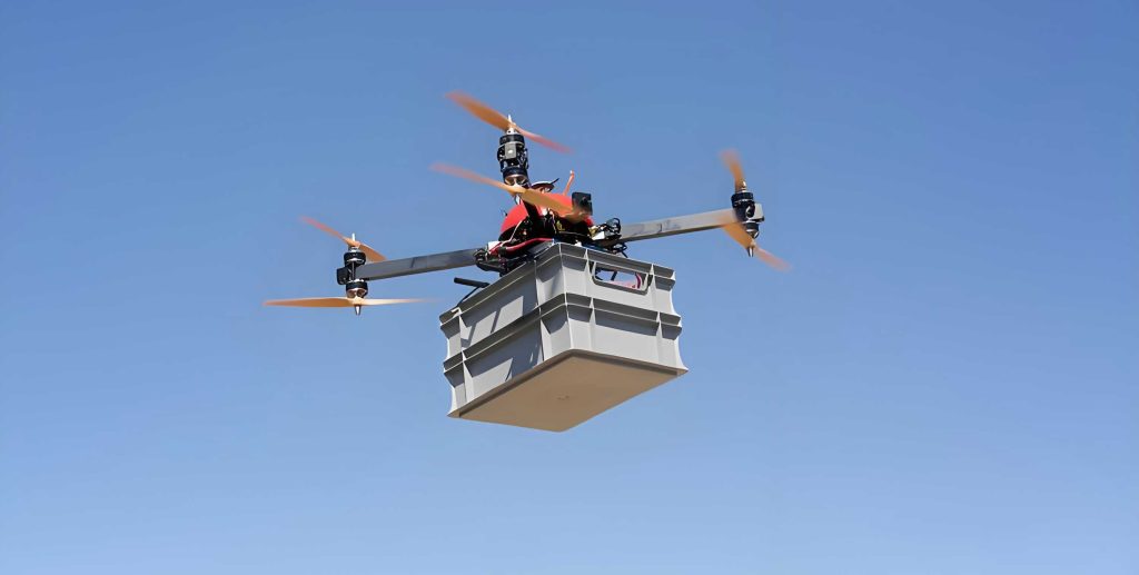
Jamming recognition for UAV communication links faces three major challenges: high noise levels obscure the weak distinguishing features of different jamming types, multidimensional features extracted from raw signals are often redundant and overlapping in feature space, and deep neural network models tend to degrade when confronted with non-stationary interference. Traditional approaches based on maximum likelihood or hand-crafted features require strong prior knowledge or fail under low jamming-to-noise ratio conditions. Meanwhile, convolutional neural networks achieve high accuracy in many classification tasks, but their fixed receptive fields may not capture the global dependencies present in jamming signals. To address these issues I propose a coherent pipeline that first denoises the received signal with an improved singular spectrum analysis algorithm, then selects a compact feature subset using a novel filter-based criterion, and finally classifies the selected features with an attention-enhanced convolutional neural network.
Signal Model and Problem Statement
In a typical UAV air-to-ground communication scenario, the ground station receives a combination of the desired UAV signal, jamming signals, and ambient noise. I model the received discrete baseband signal as:
$$\[
y(n) = h x(n) + k_j j(n) + w(n)
\]$$
where \(x(n)\) is the transmitted communication signal, \(j(n)\) is the jamming signal, \(w(n)\) is additive white Gaussian noise with zero mean and variance \(\sigma_w^2\), and \(h\), \(k_j\) denote the channel gains for the desired and interference paths respectively. I focus on ten common suppression jamming types that are frequently encountered in UAV air-to-ground links: continuous wave (CW), amplitude modulation (AM), noise amplitude modulation (NAM), binary phase shift keying (BPSK), binary frequency shift keying (BFSK), partial band noise jamming (PBNJ), multi-tone jamming (MTJ), linear frequency modulation (LFM), noise frequency modulation (NFM), and periodic pulse noise jamming (PPNJ). Their mathematical representations are summarized in Table 1.
| Jamming type | Time-domain expression | Key parameters |
|---|---|---|
| CW | \(J(t)=U_0\cos(2\pi f_I t+\theta_I)\) | \(U_0\), \(f_I\), \(\theta_I\) |
| AM | \(J(t)=U_0[1+\beta_{AM} \cos(2\pi f_m t+\theta_m)]\cos(2\pi f_I t+\theta_I)\) | \(\beta_{AM}\), \(f_m\), \(f_I\) |
| NAM | \(J(t)=[U_0+U_n(t)]\cos(2\pi f_I t+\theta_I)\) | \(U_n(t)\): band-limited white Gaussian noise |
| BPSK | \(J(t)=U_0\cos(2\pi f_I t+\theta_I+\theta_P)\), \(\theta_P\in\{0,\pi\}\) | \(\theta_P\): BPSK phase |
| BFSK | \(J(t)=U_0\cos(2\pi f_{I,1} t+\theta_I)\) or \(U_0\cos(2\pi f_{I,2} t+\theta_I)\) | \(f_{I,1}, f_{I,2}\): two frequencies |
| PBNJ | \(J(t)=U_n(t)\cos(2\pi f_I t+\theta_I)\) | Band-limited noise with variance \(\sigma_n^2\) |
| MTJ | \(J(t)=\sum_{i=1}^{N} U_0^{(i)}\cos(2\pi f_I^{(i)} t+\theta_I^{(i)})\) | \(N\) tones |
| LFM | \(J(t)=U_0\cos\left(2\pi f_I t + 2\pi \frac{f_H-f_L}{2 T_{sweep}} t^2 + \theta_I\right)\) | \(f_H, f_L, T_{sweep}\) |
| NFM | \(J(t)=U_0\cos\left(2\pi f_I t + 2\pi K_{FM} \int_0^t U_n(\tau) d\tau + \theta_I\right)\) | \(K_{FM}\): modulation index |
| PPNJ | \(J(t)=\begin{cases} U_n(t), & kT \le t \le kT+\tau \\ 0, & \text{otherwise} \end{cases}\) | Period \(T\), duty cycle \(\alpha=\tau/T\) |
The objective of this research is to classify these ten jamming signals reliably when the jamming-to-noise ratio varies from \(-20\) to \(20\) dB. I define the jamming-to-noise ratio as:
$$\[
\mathrm{JNR}=10\log_{10} \frac{P_j}{P_w}
\]$$
where \(P_j\) is the average power of the jamming signal and \(P_w\) is the noise power. At low JNR, the jamming signals are nearly hidden in noise, which makes the classification task extremely challenging. A robust preprocessing stage is therefore indispensable for improving the quality of the features fed into the classifier.
Proposed Multistep Singular Spectrum Analysis Filtering
Singular spectrum analysis is a well-known nonparametric technique for denoising and extracting trends from time series. The classical SSA first constructs a trajectory matrix from the one-dimensional signal. For a signal \(x(n)\), \(n=1,\ldots,N\), with window length \(K\), the Hankel trajectory matrix is:
$$\[
\mathbf{X}=
\begin{pmatrix}
x_1 & x_2 & \cdots & x_K \\
x_2 & x_3 & \cdots & x_{K+1} \\
\vdots & \vdots & \ddots & \vdots \\
x_{L} & x_{L+1} & \cdots & x_N
\end{pmatrix}
\]$$
where \(L=N-K+1\). The SVD of \(\mathbf{X}\) yields the eigenvectors and eigenvalues that are used to reconstruct a denoised signal by selecting the first \(p\) principal components. The main drawback of SSA is its high computational cost, especially when \(N\) is large, because the trajectory matrix has dimensions \(L \times K\) and SVD is an expensive operation. To mitigate this, I propose the multistep singular spectrum analysis (MS-SSA) algorithm. In MS-SSA, the trajectory matrix is constructed with a delay step \(S\), so the matrix becomes:
$$\[
\mathbf{X}_S=
\begin{pmatrix}
x_1 & x_2 & \cdots & x_K \\
x_{1+S} & x_{2+S} & \cdots & x_{K+S} \\
\vdots & \vdots & \ddots & \vdots \\
x_{1+(L-1)S} & x_{2+(L-1)S} & \cdots & x_{K+(L-1)S}
\end{pmatrix}
\]$$
where the number of rows is now:
$$\[
L_S = \left\lfloor \frac{N-K}{S} \right\rfloor + 1
\]$$
Thus increasing \(S\) reduces the size of the trajectory matrix and consequently the computational burden of SVD. The filtering procedure first computes the covariance matrix \(\mathbf{X}_S \mathbf{X}_S^T\), performs eigendecomposition, and retains only those components whose cumulative energy exceeds a threshold \(\eta\). The reconstruction is accomplished by a generalized slanted-diagonal averaging formula. Given a matrix \(\mathbf{Y} = (y_{i,j})\) with \(i=1,\ldots,L_S\) and \(j=1,\ldots,K\), the reconstructed time series \(\hat{x}(t)\) is obtained by averaging along the slanted diagonals defined by the step \(S\). I derived the reconstruction formula as:
For \(1 \le t \le L_S\):
$$\[
\hat{x}(t) = \frac{1}{\lceil t/S \rceil} \sum_{m=1}^{\lceil t/S \rceil} y_{m,\, t – (m-1)S}
\]$$
For \(L_S < t < K\):
$$\[
\hat{x}(t) = \frac{1}{\lceil t/S \rceil} \sum_{m=1}^{\lceil t/S \rceil} y_{\lceil t/S \rceil – m + 1,\, t – (\lceil t/S \rceil – m)S}
\]$$
For \(K \le t \le N\):
$$\[
\hat{x}(t) = \frac{1}{\lfloor (N-t)/S \rfloor + 1} \sum_{m=1}^{\lfloor (N-t)/S \rfloor + 1} y_{L_S – m + 1,\, t – (L_S – m)S}
\]$$
These formulas make it possible to reconstruct a full-length sequence from the reduced trajectory matrix.
To reduce the computational load even further when the delay step \(S\) is small, I propose the matrix-extension-based multistep SSA (MEMS-SSA). In MEMS-SSA, the reduced trajectory matrix is expanded by inserting \(S-1\) rows of zeros between each pair of consecutive rows. This expansion produces a matrix with the same size as the Hankel matrix of classic SSA. The zero-padded matrix is then subjected to the same SVD and grouping steps. Because the zeros do not contribute to the signal components, the reconstruction can be performed efficiently using the sparse structure. The complexity analysis indicates that the classic SSA requires \(O(K^3)\) operations for SVD when \(L \approx K\), while MS-SSA requires \(O(K^2 L_S)\) operations, which is substantially smaller for \(S>1\). In addition, the reconstruction complexity of MS-SSA is comparable to classic SSA because the number of non-zero entries is proportional to the actual data length.
I evaluated the computational complexity in terms of execution time (ET) and memory usage (MU). Table 2 compares the three algorithms for a sequence of length \(N=3000\), window length \(K=1000\), and varying \(S\).
| Algorithms | S | MU (MiB) | ET (s) |
|---|---|---|---|
| SSA | 1 | 22408.7 | 89.316 |
| MS-SSA | 20 | 257.9 | 13.598 |
| MS-SSA | 50 | 149.0 | 3.062 |
| MS-SSA | 100 | 129.8 | 1.135 |
| MS-SSA | 200 | 124.1 | 0.453 |
| MEMS-SSA | 20 | 288.8 | 6.582 |
| MEMS-SSA | 50 | 178.8 | 2.692 |
| MEMS-SSA | 100 | 159.8 | 1.375 |
| MEMS-SSA | 200 | 154.5 | 0.714 |
As shown, MS-SSA reduces the execution time by two or three orders of magnitude compared with the classic SSA. The filtering performance evaluated by root mean square error is also improved. For instance, at JNR = 0 dB, the RMSE of the noisy signal is 0.1008. After MS-SSA filtering with \(S=100\), the RMSE drops to 0.0442, whereas the classic SSA gives an RMSE of 0.1333. This result confirms that the proposed MS-SSA not only is faster but also yields better denoising performance for UAV interference signals.
Data processing pipeline for UAV jamming signals
Based on the MS-SSA filter, I construct a complete data processing pipeline for the received UAV jamming signals. The steps are summarized below.
- Preprocessing: The received signal \(y(n)\) is first normalized to zero mean and unit variance to remove amplitude dependencies. This is done by computing \(\hat{x}(n) = (x(n)-\mu)/\sigma\), where \(\mu\) and \(\sigma\) are the mean and standard deviation of the original signal.
- Segmentation: The normalized signal is divided into overlapping windows of length \(W\) with slide distance \(S_{slide}\). In my experiments \(W=3000\) and \(S_{slide}=100\). This segmentation increases the number of training samples and helps the filter exploit local stationarity.
- Filtering: Each segment is processed by the MS-SSA algorithm with window length \(K=1000\), step \(S=100\), and threshold \(\eta=0.85\). The filtered segments are then concatenated to form the denoised signal matrix.
- Feature extraction: From each denoised segment, I extract a set of hand-crafted features from time domain, frequency domain, and other domains. These features are carefully selected to capture the distinctive signatures of the ten jamming types.
The extracted features include: time-domain envelope fluctuation \(R = \sigma^2/\mu^2\), time-domain skewness, time-domain kurtosis, frequency-domain kurtosis, frequency-domain peak-to-average ratio, high-order peak energy concentration, average spectrum flatness, carrier factor, power spectrum variation coefficient, power spectrum entropy, fractional Fourier energy concentration, and cosine similarity coefficient. I denote the complete feature vector as \(\mathbf{F} = [F_1,F_2,\ldots,F_f]^T\). The raw feature dimension is \(f=17\).
Before feeding the feature vector into a classifier, I apply a feature selection step to reduce redundancy and improve inter-class separation. The next section describes the proposed selection criterion.
Feature Selection Using Divergence–Pearson Correlation
High-dimensional feature spaces often contain redundant or irrelevant features that degrade classification performance and increase computational cost. I propose a filter-based feature selection algorithm, called divergence–Pearson correlation coefficient feature selection (DPCC-FS), to select a compact yet discriminative subset. The algorithm combines two measures: the class separability measure based on within-class and between-class scatter matrices, and the linear correlation measure based on the Pearson correlation coefficient. The within-class scatter matrix and between-class scatter matrix are defined as:
$$\[
\mathbf{S}_w = \sum_{k=1}^{K_c} \sum_{x \in D_k} (x-\mu_k)(x-\mu_k)^T
\]$$
$$\[
\mathbf{S}_b = \sum_{k=1}^{K_c} n_k (\mu_k-\mu)(\mu_k-\mu)^T
\]$$
where \(K_c\) is the number of classes, \(D_k\) is the set of samples belonging to class \(k\), \(n_k\) is the number of samples in that class, \(\mu_k\) is the class mean, and \(\mu\) is the overall mean. The class separability criterion is:
$$\[
J_1 = \frac{\mathrm{tr}[\mathbf{S}_b]}{\mathrm{tr}[\mathbf{S}_w]}
\]$$
Larger \(J_1\) indicates better separability. The Pearson correlation coefficient between two features \(f_i\) and \(f_j\) is:
$$\[
\mathrm{Corr}(f_i,f_j) = \frac{\mathrm{cov}(f_i,f_j)}{\sqrt{\mathrm{var}(f_i)\mathrm{var}(f_j)}}
\]$$
To select a feature that has high relevance with the class labels while having low redundancy with already selected features, I construct the evaluation function:
$$\[
\mathrm{DPCC}(f_i) = \alpha \frac{\mathrm{tr}[\mathbf{S}_b(f_i)]}{\mathrm{tr}[\mathbf{S}_w(f_i)]} + \beta \left(1-\max_{f_s \in \mathbf{S}} \left| \mathrm{Corr}(f_i,f_s) \right|\right)
\]$$
where \(\alpha=\beta=0.5\), \(\mathbf{S}\) is the set of selected features, and the second term penalizes high correlation with the chosen features. The DPCC-FS algorithm starts with the feature having the maximum \(J_1\). Then it iteratively adds the feature with the largest DPCC value until a predefined number of features is selected or no further improvement is observed. Algorithm 1 summarizes the procedure.
| Algorithm 1 DPCC-FS |
| Input: Data set \(\{x_i,y_i\}_{i=1}^n\), feature set \(F=\{f_1,\dots,f_d\}\), number of desired features \(d^*\) Output: Selected feature subset \(\mathbf{S}\) Initialize \(\mathbf{S} = \emptyset\), \(T = F\) For each feature \(f \in T\) compute \(J_1(f)\) and pick \(f^* = \arg\max_f J_1(f)\) \(\mathbf{S} \leftarrow \mathbf{S} \cup \{f^*\}\), \(T \leftarrow T \setminus \{f^*\}\) while \(|\mathbf{S}| < d^*\) do for each \(f_i \in T\) compute \(\mathrm{DPCC}(f_i)\) using \(\mathbf{S}\) choose \(f_j = \arg\max \mathrm{DPCC}\) if \(\mathrm{DPCC}(f_j) > 0\) then \(\mathbf{S} \leftarrow \mathbf{S} \cup \{f_j\}\) \(T \leftarrow T \setminus \{f_j\}\) end while return \(\mathbf{S}\) |
I applied DPCC-FS to the seventeen extracted features. The selected optimal subset contained eight features: time-domain envelope fluctuation, frequency-domain kurtosis, high-order peak energy concentration, average spectrum flatness, carrier factor, power spectrum variation coefficient, power spectrum entropy, and fractional Fourier energy concentration. The reduced feature set preserves the most discriminative information while removing redundant features, thereby improving both speed and accuracy of the downstream classifier.
Channel–Space Attention Convolutional Neural Network
Deep convolutional neural networks have demonstrated great success in many classification tasks, but they tend to suffer from performance degradation when trained on small or noisy datasets. Multi-branch networks have been used to improve accuracy, yet they often increase computational cost and memory consumption. To overcome these limitations, I design the channel-space attention convolutional neural network (CSA-CNN). The core of CSA-CNN is a channel-space attention mechanism that adaptively recalibrates the feature maps in two dimensions: channel and spatial.
Channel attention
Channel attention computes a weighting vector that assigns different importance to different feature channels. I adopt a design that uses both max pooling and average pooling to capture the most salient and the average statistics of each channel. Given an intermediate feature map \(\mathbf{F} \in \mathbb{R}^{C \times H \times W}\), the channel attention weights are:
$$\[
\mathbf{W}_c = \sigma\left( \mathrm{Conv}_{3\times3} \left( \mathrm{Concat}\left[ \mathrm{MaxPool}(\mathbf{F}), \mathrm{AvgPool}(\mathbf{F}) \right] \right) \right)
\]$$
where \(\sigma\) is the Sigmoid activation. The channel-refined feature is \(\mathbf{F}_c = \mathbf{W}_c \otimes \mathbf{F}\).
Spatial attention
Spatial attention emphasizes important spatial locations. I also leverage both max pooling and average pooling along the channel dimension to generate two spatial feature descriptors, which are concatenated and passed through a convolution layer to produce the spatial attention map:
$$\[
\mathbf{W}_s = \sigma\left( \mathrm{Conv}_{3\times3} \left( \mathrm{Concat}\left[ \mathrm{MaxPool}_c(\mathbf{F}), \mathrm{AvgPool}_c(\mathbf{F}) \right] \right) \right)
\]$$
The final attention output is \(\mathbf{F}_{\text{CSA}} = \mathbf{W}_s \otimes \mathbf{F}_c\). This joint attention mechanism helps the network focus on the most discriminative parts of the jamming features.
The overall CSA-CNN architecture consists of multiple encoder–decoder blocks. Each encoder block contains a convolutional layer, batch normalization, ReLU activation, and a CSA module. A decoder block restores the resolution by combining the high-level features with the original features through residual connections. The residual connections prevent gradient vanishing and mitigate the degradation problem. The final classification is performed by a global average pooling layer followed by a fully connected layer and a softmax operation. The softmax output gives the probability distribution over the ten jamming classes:
$$\[
\hat{y}_k = \frac{\exp(z_k)}{\sum_{j=1}^{10} \exp(z_j)}
\]$$
where \(z_k\) is the logit for class \(k\). The network is trained by minimizing the categorical cross-entropy loss:
$$\[
\mathcal{L} = -\sum_{k=1}^{10} y_k \log \hat{y}_k
\]$$
I employ Adam optimization with an initial learning rate of 0.001 and a mini-batch size of 1000. The complete model architecture is listed in Table 3.
| Layer | Output shape | Configuration |
|---|---|---|
| Input | \(8 \times 1\) | Selected feature vector |
| Reshape | \(8 \times 1 \times 1\) | – |
| Conv1 | \(8 \times 1 \times 32\) | \(3\times1\), ReLU, BN |
| CSA1 | \(8 \times 1 \times 32\) | Channel+spatial attention |
| Conv2 | \(8 \times 1 \times 64\) | \(3\times1\), ReLU, BN |
| CSA2 | \(8 \times 1 \times 64\) | Channel+spatial attention |
| Encoder block | \(4 \times 1 \times 128\) | Conv + MaxPool |
| Decoder block | \(8 \times 1 \times 128\) | Upsampling + residual + CSA |
| Global average pooling | 128 | – |
| Fully connected | 10 | Softmax |
The proposed CSA-CNN has only \(2\) encoder–decoder layers, which keeps the computational cost low while still benefiting from the attention mechanism. The residual connections are implemented by adding the pre-attention feature maps to the post-convolution outputs. This design effectively solves the model degradation problem that often occurs in deep convolutional networks.
Experimental Verification
Dataset construction and simulation setup
I evaluate the proposed methods using both simulated signals and a real-world data set collected with a UAV-to-ground software-defined radio testbed. The simulation environment follows the signal models in Table 1, with the carrier frequency centered around \(2.4\) GHz and a sampling frequency of \(10\) GHz. The jamming-to-noise ratio varies from \(-20\) to \(20\) dB in steps of \(2\) dB. At each JNR, I generate \(200\) samples for each jamming type, giving a total of \(21 \times 200 \times 10 = 42000\) samples. The real-world data set is collected by a USRP B210 transmitter aboard a UAV and an ANTSDR E310 receiver on the ground. The communication link uses QPSK modulation with a Barker-13 spreading code. The jamming signals are transmitted from an additional USRP device. The measured data set contains the ten jamming types at five different jamming power levels, with \(2000\) samples per type per power level.
All experiments are repeated five times to compute the average recognition accuracy. I compare the proposed CSA-CNN with a standard CNN and a multi-branch CNN (MB-CNN). For fair comparison, the same training/test split is used throughout (50% training, 50% testing).
Hyperparameter analysis
I first analyze the effect of the number of encoder-decoder layers and batch size on the recognition accuracy at different JNRs. The results are shown in Table 4. The accuracy is averaged over five independent runs. From the table, a model with two layers and batch size \(1000\) yields the best trade-off between accuracy and computational cost. Increasing the number of layers to four degrades performance in the low-JNR regime due to overfitting. Therefore, I set the number of layers to \(2\) in all subsequent experiments.
| Layers | Batch Size | JNR=-20 | JNR=-10 | JNR=0 | JNR=10 | JNR=20 |
|---|---|---|---|---|---|---|
| 1 | 500 | 43.8 | 78.1 | 92.8 | 99.9 | 100.0 |
| 1 | 1000 | 42.8 | 78.4 | 94.4 | 99.9 | 100.0 |
| 2 | 500 | 44.8 | 78.1 | 95.4 | 99.8 | 100.0 |
| 2 | 1000 | 46.8 | 80.2 | 96.3 | 100.0 | 100.0 |
| 2 | 1500 | 47.5 | 78.3 | 94.4 | 99.9 | 100.0 |
| 3 | 1000 | 44.8 | 77.1 | 90.7 | 99.9 | 100.0 |
| 4 | 1000 | 43.8 | 77.9 | 89.2 | 98.7 | 100.0 |
Effect of MS-SSA filtering on recognition accuracy
To assess the benefit of using the proposed MS-SSA preprocessing, I run CSA-CNN on both the unfiltered and the filtered feature data sets. Table 5 presents the average accuracy values over JNR \(-20\) dB to \(20\) dB for the three models. The results demonstrate that MS-SSA filtering consistently improves the recognition accuracy. For example, the average accuracy of CSA-CNN increases from \(79.731\%\) (unfiltered) to \(82.981\%\) (filtered), which is a relative improvement of about \(4\%\). The improvement is more pronounced for low JNR values.
| Model | Unfiltered (%) | Filtered (%) |
|---|---|---|
| CNN | 73.788 | 76.906 |
| MB-CNN | 76.675 | 78.725 |
| CSA-CNN | 79.731 | 82.981 |
Comparison of recognition performance
Table 6 reports the detailed accuracy of the three models on the filtered dataset for JNR values from \(-20\) dB to \(20\) dB. The proposed CSA-CNN achieves the highest accuracy in almost every scenario. When JNR \(\ge 8\) dB, CSA-CNN reaches \(100\%\) classification accuracy. Even at JNR = \(-20\) dB, the proposed model attains \(46.8\%\), which is about \(4-7\%\) higher than the standard CNN and multi-branch CNN.
| JNR (dB) | CNN (%) | MB-CNN (%) | CSA-CNN (%) |
|---|---|---|---|
| -20 | 39.5 | 42.9 | 46.8 |
| -18 | 45.7 | 48.1 | 55.4 |
| -16 | 52.1 | 57.8 | 63.3 |
| -14 | 63.5 | 66.8 | 69.6 |
| -12 | 68.4 | 71.9 | 75.7 |
| -10 | 74.6 | 75.8 | 80.2 |
| -8 | 77.4 | 79.5 | 83.0 |
| -6 | 81.4 | 81.9 | 84.2 |
| -4 | 83.2 | 83.3 | 86.4 |
| -2 | 86.4 | 87.7 | 90.6 |
| 0 | 89.6 | 91.6 | 96.3 |
| 2 | 91.1 | 93.3 | 97.6 |
| 4 | 93.0 | 93.8 | 99.0 |
| 6 | 93.9 | 94.4 | 99.6 |
| 8 | 94.3 | 95.8 | 100.0 |
| 10 | 96.4 | 95.0 | 100.0 |
| 12 | 95.8 | 96.0 | 100.0 |
| 14 | 95.4 | 95.7 | 100.0 |
| 16 | 97.1 | 97.2 | 100.0 |
| 18 | 98.5 | 98.5 | 100.0 |
| 20 | 100.0 | 100.0 | 100.0 |
Effect of feature selection
I also analyze the impact of DPCC-FS on the final accuracy. Table 7 compares the results before and after feature selection. The selected feature set generally improves accuracy for all models, especially at medium JNR. For CSA-CNN, feature selection increases accuracy from \(96.3\%\) to \(96.9\%\) at JNR=0 dB, and from \(97.6\%\) to \(99.4\%\) at JNR=2 dB. At high JNR (\(\ge 10\) dB), the accuracy of CSA-CNN remains perfect, while the other models occasionally degrade slightly due to the reduced feature dimension. Overall, DPCC-FS is beneficial for the proposed model and does not sacrifice its high-JNR performance.
| JNR (dB) | CNN (no FS) | CNN (FS) | MB-CNN (no FS) | MB-CNN (FS) | CSA-CNN (no FS) | CSA-CNN (FS) |
|---|---|---|---|---|---|---|
| -20 | 39.5 | 43.3 | 42.9 | 44.6 | 46.8 | 46.8 |
| -10 | 74.6 | 77.1 | 75.8 | 81.0 | 80.2 | 82.7 |
| 0 | 89.6 | 88.8 | 91.6 | 92.9 | 96.3 | 96.9 |
| 2 | 91.1 | 90.5 | 93.3 | 94.6 | 97.6 | 99.4 |
| 10 | 96.4 | 94.4 | 95.0 | 94.8 | 100.0 | 100.0 |
| 20 | 100.0 | 100.0 | 100.0 | 100.0 | 100.0 | 100.0 |
Real-world data set evaluation
To validate the practical value of the proposed method, I use the real-world data collected from the drone-to-ground testbed. The classification results under five jamming power levels are shown in Table 8. The jamming power \(P_j\) varies from 0.01 W to 0.2 W. For each power level, the test set contains 500 samples per jamming class. The proposed CSA-CNN achieves the best performance at all power levels, reaching \(99.3\%\) accuracy at \(P_j=0.2\) W. At low jamming power, the advantage of CSA-CNN is even more evident, demonstrating its robustness in realistic weak-interference scenarios.
| Jamming power \(P_j\) (W) | CNN (%) | MB-CNN (%) | CSA-CNN (%) |
|---|---|---|---|
| 0.01 | 41.7 | 46.9 | 50.1 |
| 0.05 | 72.9 | 77.8 | 83.5 |
| 0.10 | 80.4 | 82.5 | 86.9 |
| 0.15 | 92.3 | 88.2 | 96.9 |
| 0.20 | 94.1 | 92.8 | 99.3 |
Confusion matrix analysis at low JNR
To further understand the classification behavior, I examine the confusion matrix at JNR = \(-20\) dB for the CSA-CNN model. Most confusions occur among the noise-like jamming types, particularly CW vs. NAM and PBNJ vs. PPNJ. As the JNR increases to 0 dB and beyond, the confusion disappears and the model becomes highly confident. The proposed attention mechanism helps suppress these confusions by focusing on subtle frequency-domain differences that distinguish these signals.
Conclusion
In this work, I have presented a comprehensive framework for recognizing jamming signals in UAV air-to-ground communication links. The contributions are threefold. First, I proposed the multistep singular spectrum analysis algorithm, which substantially reduces the computational cost of the classical SSA while improving filtering accuracy. Second, a divergence–Pearson correlation feature selection method was introduced to select a compact feature subset that preserves the most discriminative information for the ten jamming types. Third, I designed a channel-space attention convolutional neural network that adaptively recalibrates feature maps and mitigates model degradation through residual connections. Extensive experiments on both simulated and real-world UAV communication data demonstrate that the proposed framework achieves superior recognition accuracy across a wide JNR range, from \(-20\) dB to \(20\) dB. At JNR \(\ge 8\) dB, the CSA-CNN reaches perfect classification accuracy, and even at \(-20\) dB it outperforms conventional CNN and multi-branch CNN by a meaningful margin. The combined DPCC-FS and CSA-CNN approach also maintains high robustness in realistic weak-interference environments. Future work will extend the framework to include smart jamming and compound jamming types, as well as consider the uplink direction where the ground station transmits to the UAV. I believe that the proposed methods provide a solid basis for adaptive anti-jamming decision-making in future low-altitude UAV networks.