
In this thesis, I investigate the problem of formation control for a team of unmanned aerial vehicles (UAVs) from the perspective of differential game theory. The core idea is to model each vehicle as an independent decision maker whose local control objectives, such as minimizing formation errors and energy consumption, are embedded into a dynamic game framework. By solving the corresponding Nash equilibrium, I obtain optimal control laws that enable the whole formation to achieve coordinated motion under various adverse conditions. I first review the theoretical foundations, including differential games, control barrier functions, graph theory, and memory event-triggered mechanisms. Then, I propose a hierarchical anti-attack control architecture for UAVs subject to mixed cyber attacks. In this framework, Q-learning is used to train an attack mitigation policy, while a control barrier function is incorporated to guarantee collision-free behavior. Next, I develop a cooperative control strategy that combines switching topology design, sliding-mode disturbance observers, memory event-triggered communication, and differential-game-based Nash equilibrium solving. This strategy addresses wake interference, limited communication resources, and robustness issues in multi-UAV formation flight. Through numerical simulations, I verify that the proposed methods can achieve stable and safe formation control under both cyber-physical attacks and realistic aerodynamic disturbances. I also provide a detailed convergence analysis and show that the closed-loop system can be exponentially stable under the designed memory event-triggered sliding mode controller.
The motivation for this work arises from the fact that modern civilian and military applications increasingly rely on unmanned aerial vehicles to perform complex tasks such as cooperative surveillance, search and rescue, and environmental monitoring. Compared with a single UAV, a multi-UAV formation can provide higher efficiency, broader coverage, and greater robustness. However, formation control is still a challenging problem because each vehicle is an autonomous agent with its own dynamics and local information. The conflict between individual objectives and global formation objectives makes the problem particularly suitable for differential game theory. In a differential game, the time evolution of the system is described by differential equations, and each player tries to optimize a personal performance index. The solution of the game, namely the Nash equilibrium, gives a set of control policies from which no single player can unilaterally deviate to improve its own payoff.
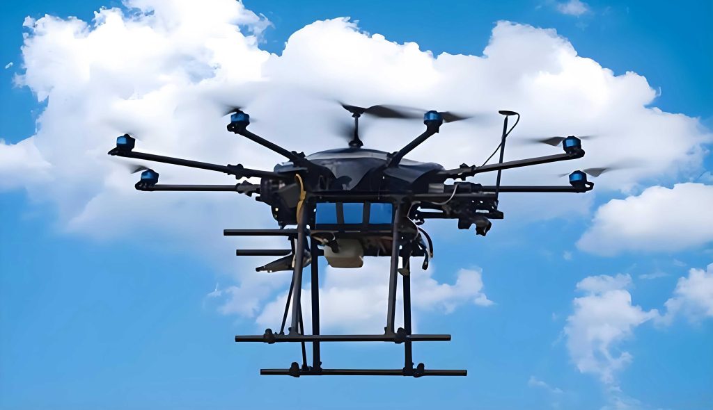
A critical issue in formation control of unmanned aerial vehicles is the presence of external disturbances and malicious attacks. In this thesis, I consider two representative cyber attacks: denial-of-service (DoS) attacks and false data injection (FDI) attacks. DoS attacks block the communication or control channels, whereas FDI attacks inject malicious data into the system. The coexistence of these attacks is more realistic than a single attack model, and it is necessary to design a control law that is resilient to both types of threats. I formulate the anti-attack problem as a zero-sum differential game in which the controller and the attacker have opposite objectives. The controller seeks to minimize a quadratic cost function, while the FDI attack input tries to maximize the same cost. I derive the optimal control input and the worst-case FDI input using dynamic programming and Riccati equations. In addition, I use Q-learning to solve the game in a model-free manner, which is useful when the system matrices are not exactly known.
Another central topic of this thesis is the safety of the formation. During formation flight, the distance between any two unmanned aerial vehicles must remain above a safe threshold. I employ control barrier functions (CBFs) to enforce this requirement. A CBF is a continuous differentiable scalar function that maps the safety constraint to an inequality condition on the control input. By adding the CBF constraint to the optimal control problem, I can ensure that the system state never leaves the safe set. In the mixed-attack environment, the CBF provides an additional layer of protection, so that even if the cyber layer is compromised, physical collisions are still avoided.
Besides security and safety, communication efficiency is another major concern in multi-UAV formation control. Since the formation relies on wireless links to exchange state information, a high communication frequency leads to unnecessary energy consumption and bandwidth occupation. To reduce the communication burden, I introduce an improved memory event-triggered mechanism (METM). Unlike the traditional event-triggered mechanism that only uses the current error, the proposed METM incorporates historical transmission data and a dynamic trigger threshold. This yields a more reasonable triggering decision and reduces the number of data transmissions while preserving the desired control performance. Combined with sliding mode control, the METM is used to design a robust controller that can compensate for communication delays and wake disturbances. I prove that the closed-loop system is exponentially stable under the proposed scheme.
The remainder of this thesis is organized as follows. In Section 2, I briefly review the necessary mathematical tools, including differential games, Q-learning, control barrier functions, graph theory, and the memory event-triggered mechanism. In Section 3, I present the first main contribution: a hierarchical control framework for safe cooperative control of unmanned aerial vehicles under mixed attacks. In Section 4, I present the second main contribution: a differential-game-based formation control strategy that integrates switching topology, sliding-mode disturbance observers, and a memory event-triggered sliding mode controller. Finally, Section 5 summarizes the results and discusses possible directions for future research.
Preliminaries and Problem Formulation
Differential Game Theory
Differential game theory is a branch of dynamic game theory that studies multi-player decision problems in continuous time. A general N-player differential game can be described by the state equation
$$ \dot{x}_i(t) = f_i\big(x(t), u_1(t), \dots, u_N(t), t\big), \quad i = 1, \dots, N, $$
where $x(t) = [x_1^T(t), \dots, x_N^T(t)]^T$ is the concatenated state vector, $u_i(t) \in U_i$ is the control strategy of player $i$, and $f_i(\cdot)$ is a continuously differentiable function. The performance index of player $i$ is given by
$$ J_i(u_1, \dots, u_N) = \phi_i(x(T)) + \int_{t_0}^{T} L_i\big(x(\tau), u_1(\tau), \dots, u_N(\tau)\big) d\tau, $$
where $x(T)$ is the terminal state, $\phi_i$ is the terminal cost, and $L_i$ is the running cost. A strategy profile $(u_1^*, \dots, u_N^*)$ is called a Nash equilibrium if for every player $i$ and every admissible strategy $u_i \in U_i$,
$$ J_i(u_1^*, \dots, u_{i-1}^*, u_i, u_{i+1}^*, \dots, u_N^*) \ge J_i(u_1^*, \dots, u_{i-1}^*, u_i^*, u_{i+1}^*, \dots, u_N^*). $$
This property makes differential games particularly attractive for formation control, because each UAV in the formation can be seen as a player that aims to minimize its own formation error and energy consumption, while taking into account the strategies of the other UAVs. In this thesis, I focus on both zero-sum games and non-cooperative games with Nash equilibrium solutions.
Control Barrier Function
A control barrier function is used to guarantee safety. Let $\mathcal{C}$ be a safe set defined by
$$ \mathcal{C} = \{ x \in \mathbb{R}^n \mid h(x) \ge 0 \}, $$
where $h: \mathbb{R}^n \to \mathbb{R}$ is a continuously differentiable function. The function $h$ is called a control barrier function for the system $\dot{x} = f(x) + g(x)u$ if there exists an extended class $\mathcal{K}_\infty$ function $\gamma$ such that
$$ \sup_{u \in U} \left[ L_f h(x) + L_g h(x) u + \gamma(h(x)) \right] \ge 0, \quad \forall x \in \mathcal{C}, $$
where $L_f h(x) = \frac{\partial h}{\partial x} f(x)$ and $L_g h(x) = \frac{\partial h}{\partial x} g(x)$. The inequality above is often used as a constraint in quadratic programming to compute a safe control input that is as close as possible to a nominal controller. In formation control, the relative distance between UAV $i$ and UAV $j$ can be protected by defining
$$ h_{ij}(x) = \| p_i – p_j \|^2 – d_{safe}^2, $$
with $d_{safe}$ being the minimum allowed distance. The constraint $h_{ij}(x) \ge 0$ ensures collision avoidance.
Graph Theory and Communication Topology
The communication topology of a multi-UAV formation is modeled by an undirected graph $\mathcal{G} = (\mathcal{V}, \mathcal{E})$, where $\mathcal{V} = \{1, 2, \dots, N\}$ is the node set and $\mathcal{E} \subseteq \mathcal{V} \times \mathcal{V}$ is the edge set. The adjacency matrix $A = [a_{ij}]$ is defined by $a_{ij} = 1$ if $(i,j) \in \mathcal{E}$ and $a_{ij} = 0$ otherwise. The Laplacian matrix $L = [l_{ij}]$ is defined by $l_{ij} = -a_{ij}$ for $i \neq j$, and $l_{ii} = \sum_{j \neq i} a_{ij}$. For a connected undirected graph, the Laplacian has a simple zero eigenvalue and all other eigenvalues are positive. I use the Laplacian matrix to describe the information exchange among unmanned aerial vehicles in the differential-game-based formation control problem. The graph-theoretic properties allow me to design distributed estimators and local controllers that only use neighbors’ information.
Memory Event-Triggered Mechanism
The memory event-triggered mechanism is an extension of the traditional event-triggered mechanism. It uses historical transmission data in addition to the current sampled error to decide whether a new data packet should be sent. Suppose that the sampling period is $h$ and the trigger times for UAV $i$ are $t_{k_i}^{(i)}$. Define the state-triggered error and the input-triggered error, respectively, as follows:
$$ e_{is}(t) = z_i(t_{k_i+s}^{(i)}) – z_i(m h), \quad e_i^u(t) = u_i(t_{k_i}^{(i)}) – u_i(m h), \quad t \in [m h, m h + h). $$
Let $S$ be the number of recent transmitted data points and let $u_s$ be a weight coefficient satisfying $\sum_{s=1}^{S} u_s = 1$. The triggering condition is designed as
$$ \sum_{s=1}^{S} u_s e_{is}^T(t) \Omega e_{is}(t) + \varepsilon_i e_i^{uT}(t) \Omega_1 e_i^u(t) \ge \rho_i(t) z_i^T(t) \Omega_2 z_i(t), $$
where $\varepsilon_i > 0$, $\rho_i(t)$ is an adaptive threshold, and $\Omega$, $\Omega_1$, $\Omega_2$ are positive definite matrices. The threshold $\rho_i(t)$ is updated by
$$ \rho_i(t) = \delta + \rho \exp\left( -\sigma \left\| \sum_{s=1}^{S} u_s e_{is}(t) \right\| – \omega \| e_i^u(t) \| \right), $$
with $\delta, \rho, \sigma, \omega > 0$ and $\delta + \rho \in (0,1)$. This adaptive threshold ensures that the trigger frequency is high when the errors are large and low when the errors are small. The internal dynamic variable $\tau_i(t)$ is generated by
$$ \dot{\tau}_i(t) = -\varepsilon_i \tau_i(t) + e_i^{uT}(t) \Omega_1 e_i^u(t). $$
The METM reduces unnecessary communication while avoiding the degradation of control performance caused by sudden short-term disturbances. In this thesis, I integrate the METM with sliding mode control to guarantee robustness.
Safe Cooperative Control of UAVs under Mixed Attacks
System Model and Attack Model
I consider a group of N unmanned aerial vehicles. Using feedback linearization, the nonlinear UAV dynamics can be transformed into a double-integrator form:
$$ \dot{x}_i = v_{x_i}, \quad \dot{v}_{x_i} = u_{x_i}, \quad \dot{y}_i = v_{y_i}, \quad \dot{v}_{y_i} = u_{y_i}, \quad \dot{h}_i = v_{h_i}, \quad \dot{v}_{h_i} = u_{h_i}. $$
Let $z_i = [p_i^T, v_i^T]^T$ and $u_i = [u_{x_i}, u_{y_i}, u_{z_i}]^T$. Then the linearized model is
$$ \dot{z}_i = A z_i + B u_i, $$
where $A = \begin{bmatrix} 0 & I_3 \\ 0 & 0 \end{bmatrix}$, $B = \begin{bmatrix} 0 \\ I_3 \end{bmatrix}$. For the entire formation, I write $\dot{z} = \mathcal{A} z + \mathcal{B} u$ with $\mathcal{A} = I_N \otimes A$, $\mathcal{B} = I_N \otimes B$.
The cyber attack is modeled as follows. The actual control input applied to the aircraft is
$$ \bar{u}_i(k) = a(k) u_i(k) + b(k) \psi_i(k), $$
where $a(k)$ and $b(k)$ are Bernoulli random variables indicating the occurrence of DoS and FDI attacks, respectively. Specifically, $a(k) = 0$ means that the DoS attack is successful, while $b(k) = 1$ means that FDI attack signal $\psi_i(k)$ is injected. The attack probabilities are $\Pr[a(k)=1] = \alpha$ and $\Pr[b(k)=1] = \beta$. To simplify the notation, I omit the time index $k$ in the following derivation.
Zero-Sum Differential Game for Anti-Attack Control
I formulate the interaction between the controller and the FDI attack as a zero-sum differential game. The cost function that the controller tries to minimize is
$$ J(x_k) = \mathbb{E} \left[ \sum_{i=k}^{\infty} \eta^{i-k} \left( x_i^T Q x_i + a_i u_i^T R_1 u_i – b_i \psi_i^T R_2 \psi_i \right) \right], $$
where $Q \ge 0$, $R_1 > 0$, $R_2 > 0$ are weighting matrices, and $\eta \in (0,1)$ is a discount factor. The Bellman equation for this game is
$$ J(x_k) = x_k^T Q x_k + u_k^T R_1 u_k – \psi_k^T R_2 \psi_k + \eta J(x_{k+1}). $$
Because the value function is quadratic, I set $J(x) = x^T P x$. Then the Hamiltonian is
$$ H(x,u,\psi) = x^T Q x + u^T R_1 u – \psi^T R_2 \psi + \eta x_{k+1}^T P x_{k+1} – x_k^T P x_k. $$
By applying the stationarity conditions $\frac{\partial H}{\partial u} = 0$ and $\frac{\partial H}{\partial \psi} = 0$, I obtain the worst-case FDI attack and the optimal control input as follows. First define the matrices
$$ \rho = R_1 + \eta D^T P D, \quad \theta = R_2 – \eta D^T P D. $$
Then the optimal control and the worst-case attack are given by
$$ u^* = -\rho^{-1} \left( \eta D^T P C x + \beta \eta D^T P D v^* \right), $$
$$ \psi^* = \theta^{-1} \left( -\beta \eta D^T P C x + \alpha \eta D^T P D u^* \right). $$
After substitution, the game algebraic Riccati equation (GARE) is obtained:
$$ P = Q + \eta C^T P C – \eta^2 \begin{bmatrix} \alpha C^T P D & \beta C^T P D \end{bmatrix} \begin{bmatrix} \rho & \alpha \beta \eta D^T P D \\ \alpha \beta \eta D^T P D & \beta \theta \end{bmatrix}^{-1} \begin{bmatrix} \alpha D^T P C \\ \beta D^T P C \end{bmatrix}. $$
I prove in Section 3 of the thesis that the sequence generated by iterating this Riccati equation is monotonically increasing and converges to the stabilizing solution. The conditions include
$$ \left( \frac{R_1}{\eta} – D^T P D \right) > \frac{\alpha \beta^2}{1-\beta} D^T P D, $$
and the maximum eigenvalue condition $\lambda_{\max}(\eta C C^T) \le 1$. These conditions guarantee the existence and uniqueness of the solution to the GARE.
To solve the game without requiring exact system dynamics, I use a Q-learning algorithm. The Q-function is defined as
$$ Q(z_k) = z_k^T \mathcal{M} z_k, $$
where $z_k = [x_k^T, u_k^T, \psi_k^T]^T$ and the matrix $\mathcal{M}$ is partitioned as
$$ \mathcal{M} = \begin{bmatrix} M_{11} & M_{12} & M_{13} \\ M_{21} & M_{22} & M_{23} \\ M_{31} & M_{32} & M_{33} \end{bmatrix}. $$
Using the least-squares method, the Q-matrix is updated by
$$ z_k^T \mathcal{M}^t z_k = \eta z_{k+1}^T \mathcal{M}^{t-1} z_{k+1} + x_k^T Q x_k + u_k^T R_1 u_k – \psi_k^T R_2 \psi_k. $$
The control and attack policies are then extracted from the Q-matrix:
$$ u = -\left( M_{22}^t \right)^{-1} \left( M_{21}^t x + M_{23}^t \psi \right), $$
$$ \psi = -\left( M_{33}^t – M_{32}^t (M_{22}^t)^{-1} M_{23}^t \right)^{-1} \left( M_{31}^t – M_{32}^t (M_{22}^t)^{-1} M_{21}^t \right) x. $$
Exploration noise is added to satisfy the persistence of excitation condition. The overall algorithm is summarized below.
| Step | Action |
|---|---|
| 1 | Initialize $P^{(0)} = 0$, $M^{(0)} = 0$, $K^{(0)} = 0$, $L^{(0)} = 0$. |
| 2 | Policy evaluation: solve $\mathbf{z}_k^T M^{(t)} \mathbf{z}_k = \mathbf{z}_{k+1}^T M^{(t-1)} \mathbf{z}_{k+1} + \mathbf{x}_k^T Q \mathbf{x}_k + u_k^T R_1 u_k – \psi_k^T R_2 \psi_k$ via least squares. |
| 3 | Policy improvement: update $u^{(t+1)}$ and $\psi^{(t+1)}$ using the formulas above. |
| 4 | Set $t \leftarrow t+1$ and repeat steps 2-3 until $t = t_{max}$ or $\| M^{(j+1)} – M^{(j)} \| < \epsilon$. |
Formation Control via Differential Game and CBF
After designing the anti-attack control layer, I focus on the formation control layer. I define the desired displacement vector from UAV $j$ to UAV $i$ as $\alpha_{ij}$. The performance index for UAV $i$ is
$$ J_i = \sum_{j \in \mathcal{N}_i} l_{ij} \left( \| p_i(t_f) – p_j(t_f) – \alpha_{ij} \|^2 + \| v_i(t_f) – v_j(t_f) \|^2 \right) + \int_0^{t_f} \frac{r_i}{2} \| u_i \|^2 dt, $$
where $\mathcal{N}_i$ is the neighbor set of UAV $i$, $l_{ij}$ is the entry of the Laplacian matrix, $r_i$ is a positive scalar, and $t_f$ is the terminal time. This performance index reflects that each UAV only cares about its own terminal formation error, terminal velocity error, and control effort. The resulting differential game has a Nash equilibrium solution. By introducing auxiliary state variables
$$ s_{p_i}(t) = \left( t – t_f \right) v_i(t) + p_i(t), \quad s_{v_i}(t) = v_i(t), $$
I convert the terminal cost into a quadratic cost of the auxiliary states. Using Pontryagin’s minimum principle and the Hamiltonian
$$ H_i = \frac{r_i}{2} \| u_i \|^2 + \lambda_{p_i}^T B_p u_i + \lambda_{v_i}^T B_v u_i, $$
I derive the open-loop Nash equilibrium as
$$ u_i^* = -\frac{1}{r_i} F_i \left( M^{-1} \left( W \begin{bmatrix} s_p(0) \\ s_v(0) \end{bmatrix} + R^{-1} \otimes I_3 \alpha \right) + \alpha \right), $$
where $M$ is defined in the thesis and is invertible. However, this expression requires global information, so I propose a distributed terminal state estimator. Let $\zeta_{p_i}(t)$ and $\zeta_{v_i}(t)$ be the estimates of $s_{p_i}(t)$ and $s_{v_i}(t)$, respectively. The distributed estimation law is
$$ \begin{bmatrix} \dot{\zeta}_{p_i} \\ \dot{\zeta}_{v_i} \end{bmatrix} = k_i \begin{bmatrix} w_{pp} & w_{pv} \\ w_{vp} & w_{vv} \end{bmatrix} \begin{bmatrix} \zeta_{p_i} \\ \zeta_{v_i} \end{bmatrix} + k_i \begin{bmatrix} 0 \\ I_3 \end{bmatrix} \alpha_i – k_i \sum_{j \in \mathcal{N}_i} l_{ij} \begin{bmatrix} \zeta_{p_i} – \zeta_{p_j} \\ \zeta_{v_i} – \zeta_{v_j} \end{bmatrix}, $$
where $k_i$ is a positive scalar and the weights $w_{pp}, w_{pv}, w_{vp}, w_{vv}$ are computed from the matrices $B_p, B_v$ and the weighting coefficients. I prove that the estimation errors converge to zero, i.e.,
$$ \lim_{t \to \infty} \zeta_{p_i}(t) = s_{p_i}(t), \quad \lim_{t \to \infty} \zeta_{v_i}(t) = s_{v_i}(t). $$
Then the distributed Nash control law is
$$ u_i^* = -\frac{1}{r_i} \sum_{j \in \mathcal{N}_i} l_{ij} \left( B_p^T (\zeta_{p_i} – \zeta_{p_j} – \alpha_{ij}) + B_v^T (\zeta_{v_i} – \zeta_{v_j}) \right). $$
To guarantee collision avoidance, I add a CBF constraint. The distance between UAV $i$ and UAV $j$ is $d_{ij} = \| p_i – p_j \|$. The candidate control barrier function is
$$ h_{ij} = d_{ij}^2 – d_{safe}^2. $$
According to the CBF condition, the control input must satisfy
$$ \dot{h}_{ij} + \lambda h_{ij} \ge 0, \quad \lambda > 0. $$
Since $\dot{h}_{ij} = 2 (p_i – p_j)^T (v_i – v_j)$, and the acceleration appears in the derivative, the condition is linear in the control input. I combine the nominal controller from the Nash equilibrium with the CBF constraint using a quadratic programming (QP) formulation:
$$ \min_{u} \; \| u – u^* \|^2 \quad \text{subject to } \; \dot{h}_{ij} + \lambda h_{ij} \ge 0, \; \forall i \neq j. $$
This ensures that the resulting control input is as close as possible to the game-optimal input while explicitly satisfying the safety constraint. The overall architecture is hierarchical: the lower Q-learning layer handles attacks, the middle differential game layer generates the formation control strategy, and the upper CBF-QP layer enforces safety. The numerical simulation considers five unmanned aerial vehicles with a total simulation time of 60 seconds and a sampling period of 0.05 seconds. The parameters are listed below.
| Parameter | Value |
|---|---|
| Number of UAVs | 5 |
| Mass | 20 kg |
| Gravity | $9.81 \, \mathrm{m/s^2}$ |
| Formation target time | 30 s |
| Attack probability $\alpha, \beta$ | 0.2 |
| Discount factor $\eta$ | 0.99 |
| Safe distance $d_{safe}$ | 30 m |
The simulation results show that the formation is successfully built even under mixed attacks. The 3D trajectories of the five unmanned aerial vehicles converge to the desired formation shape. The distance between every pair of UAVs remains above the safe distance, which demonstrates that the CBF constraint is effective. The Riccati matrix, controller gain, and attacker gain converge quickly, confirming the convergence of the GARE solution.
Differential Game Control of UAV Formation with Memory Event-Triggered Sliding Mode Control
Problem Statement with Wake Disturbances
In this scenario, I consider a leader-follower formation of unmanned aerial vehicles. Each follower is affected by the wake of the leader and other neighboring UAVs. The nonlinear model with wake disturbances is given by the following six state equations:
$$ \dot{x}_i = V_i \cos \gamma_i \cos \chi_i + \delta_{x_i}, \quad \dot{y}_i = V_i \cos \gamma_i \sin \chi_i + \delta_{y_i}, \quad \dot{h}_i = V_i \sin \gamma_i + \delta_{h_i}, $$
$$ \dot{V}_i = \frac{V_{i_l} – V_i}{\tau_{V_i}} + \delta_{V_i}, \quad \dot{\gamma}_i = \frac{\gamma_{i_l} – \gamma_i}{\tau_{\gamma_i}} + \delta_{\gamma_i}, \quad \dot{\chi}_i = \frac{\chi_{i_l} – \chi_i}{\tau_{\chi_i}} + \delta_{\chi_i}, $$
where $\delta_{x_i}, \delta_{y_i}, \delta_{h_i}, \delta_{V_i}, \delta_{\gamma_i}, \delta_{\chi_i}$ are the bounded wake disturbances. Using dynamic surface control and introducing pseudo-control quantities, I transform the model into strict-feedback form. Let $p_i = [x_i, y_i, h_i]^T$ and $v_i = \dot{p}_i$. Then the state-space form is
$$ \begin{aligned} \dot{p}_i &= v_i, \\ \dot{v}_i &= u_i(t) + \delta_i(t), \end{aligned} $$
where $u_i(t)$ is the virtual acceleration control and $\delta_i(t)$ is the integrated disturbance vector. In the leader-follower context, the desired formation is specified by the desired displacement $\alpha_{ij}$ from follower $j$ to follower $i$.
Switching Topology Design
To improve communication efficiency, I design a distributed topology control layer. The maximum transmission range of each UAV is assumed to be a sphere. The sphere is partitioned into $n$ equal-volume sectors, each containing the center. I choose the partition vectors as the normals of a regular polyhedron. For $n = 8$, the vectors are $(\pm 1, \pm 1, \pm 1)$. For $n = 20$, the vectors are derived from the icosahedron. The topology control algorithm works as follows.
| Step | Description |
|---|---|
| 1 | Each UAV periodically broadcasts its position vector $p_0$. |
| 2 | Each UAV receives neighbor position messages and updates the set $P$. |
| 3 | For each neighbor $p$, compute $d = p – p_0$, and find the partition vector $s^*$ maximizing $s \cdot d$. |
| 4 | Assign the neighbor to the corresponding sector. |
| 5 | For each sector, construct a minimum spanning tree (MST) including the local UAV. |
| 6 | Select the nearest neighbor from each sector and adjust transmission power accordingly. |
This method reduces the average number of communication links. In a five-UAV formation, a complete graph requires 10 links, whereas the proposed topology control reduces the average number to about 4.5 links while maintaining connectivity. Consequently, the transmission power consumption is significantly lowered.
Sliding Mode Disturbance Observer
To estimate the unknown wake disturbances, I design six independent sliding-mode disturbance observers, one for each channel. For the $x$-channel, the observer is
$$ \hat{x}_i = V_i \cos \gamma_i \cos \chi_i + \hat{\delta}_{x_i}, \quad \dot{\hat{v}}_{x_i} = -\lambda_{1} \mathrm{sig}(\hat{x}_i – x_i) + \hat{\delta}_{x_i}, \quad \hat{\delta}_{x_i} = -\lambda_{2} \mathrm{sign}(\dot{\hat{v}}_{x_i} – v_{x_i}), $$
where $\lambda_1, \lambda_2 > 0$ are observer gains, and $\mathrm{sig}(\cdot)$ and $\mathrm{sign}(\cdot)$ denote the standard sign functions. The other five observers are designed similarly. The disturbance estimates are denoted by $\hat{\delta}_{y_i}, \hat{\delta}_{h_i}, \hat{\delta}_{V_i}, \hat{\delta}_{\gamma_i}, \hat{\delta}_{\chi_i}$. In the controller design, I replace the actual disturbances by their estimates in a feedforward compensation term.
Memory Event-Triggered Sliding Mode Controller
Define the state error $z_i = z_i – z_i^d$. The sliding function is designed as
$$ \sigma_i(t) = C z_i(t) + \int_{t_k^{(i)}}^t \left[ C B K z_i(\tau) + C B_K e_i^u(\tau) \right] d\tau + \int_{t_k^{(i)}}^t C B e_i(\tau) d\tau, $$
where $C$ is selected such that $CB$ is nonsingular, $K$ is a feedback gain matrix, and $e_i = z_i(t) – z_i(t_k^{(i)})$ is the state-triggered error. Using the aggregate notation, the sliding function can be written as
$$ \sigma(t) = \mathcal{C} z(t) + \int_{t_k}^t \left[ \mathcal{C} \mathcal{B} \mathcal{K} z(\tau) + \mathcal{C} \mathcal{B} e(\tau) \right] d\tau. $$
The equivalent control law is derived from $\dot{\sigma}(t) = 0$:
$$ u_{eq}(t) = -(\mathcal{C} \mathcal{B})^{-1} \left( \mathcal{C} \mathcal{A} z(t) + \mathcal{C} \mathcal{B} \mathcal{K} z(t) – \mathcal{C} \mathcal{B} e(t) \right). $$
I propose the following sliding mode control law:
$$ u(t) = -(\mathcal{C} \mathcal{B})^{-1} \left( \mathcal{C} \mathcal{A} z(t) + \mathcal{C} \mathcal{B} \mathcal{K} z(t) – \mathcal{C} \mathcal{B} e(t) + \theta \, \sigma(t) + \kappa \, \mathrm{sign}(\sigma(t)) \right), $$
where $\theta > 0$ and $\kappa > 0$. The reaching condition is verified:
$$ \sigma^T(t) \dot{\sigma}(t) \le -\theta \| \sigma(t) \|^2 – \kappa \| \sigma(t) \| < 0. $$
Thus, the sliding surface is reachable in finite time. On the sliding surface, the closed-loop dynamics are governed by the reduced-order system
$$ \dot{z}(t) = \left( \mathcal{A}_1 + \mathcal{B}_1 \mathcal{K} \right) z(t) – \mathcal{B}_1 e(t) + \mathcal{B}_e e^u(t), $$
where $\mathcal{A}_1, \mathcal{B}_1, \mathcal{B}_e$ are aggregate matrices defined in the thesis. To prove exponential stability, I construct a Lyapunov–Krasovskii functional that incorporates the memory event-triggered errors. The main theorem provides a sufficient condition in terms of linear matrix inequalities (LMIs).
Let $\lambda_1$ and $\lambda_N$ be the smallest and largest eigenvalues of the Laplacian matrix $H$ of the communication graph. Define the following block matrices. The LMI condition is
$$ \begin{bmatrix} \Xi_{11} & \Xi_{12} & \cdots & \Xi_{17} \\ * & \Xi_{22} & \cdots & \Xi_{27} \\ \vdots & & \ddots & \vdots \\ * & * & \cdots & \Xi_{77} \end{bmatrix} < 0, $$
where the entries depend on the parameters and Lyapunov matrices. I list the explicit entries in the thesis. The theorem states that if there exist matrices $P > 0$, $Q > 0$, $R > 0$, $\Omega > 0$, $\Omega_1 > 0$, $Y_1$, $Y_2$, and $X = P^{-1}$ such that the LMI is feasible, then the closed-loop system is exponentially stable. The controller gain is $K = Y_1 X^{-1}$, and the trigger matrix is $\Omega = X^T \Omega X$. The proof uses a Lyapunov–Krasovskii functional of the form
$$ V(t) = z^T(t) P z(t) + \int_{t-\tau}^t e^{2\alpha (s-t)} z^T(s) Q z(s) ds + \int_{-\tau}^0 \int_{t+\theta}^t e^{2\alpha (s-t)} \dot{z}^T(s) R \dot{z}(s) ds d\theta + \text{trigger-related terms}. $$
By showing that $\dot{V}(t) + 2 \alpha V(t) \le 0$, the exponential stability with decay rate $\alpha$ is established. The detailed derivation is omitted here for brevity.
Nash Equilibrium of the Formation Differential Game
After the robust sliding mode controller stabilizes the tracking error, I formulate the formation control problem as an $N$-player differential game. The performance index for UAV $i$ is now defined with the actual control input $u_i$ and the estimated disturbance compensation:
$$ J_i = \sum_{j \in \mathcal{N}_i} l_{ij} \left( \| p_i(t_f) – p_j(t_f) – \alpha_{ij} \|^2 + \| v_i(t_f) – v_j(t_f) \|^2 \right) + \int_{0}^{t_f} \frac{r_i}{2} \| u_i \|^2 dt. $$
The Hamiltonian is
$$ H_i = \frac{r_i}{2} \| u_i \|^2 + \lambda_{p_i}^T B_p u_i + \lambda_{v_i}^T B_v u_i. $$
From the necessary conditions, I derive the optimal control as
$$ u_i^* = -\frac{1}{r_i} \left[ B_p^T \lambda_{p_i} + B_v^T \lambda_{v_i} \right]. $$
The costate variables satisfy $\dot{\lambda}_{p_i} = 0$ and $\dot{\lambda}_{v_i} = 0$ with terminal conditions
$$ \lambda_{p_i}(t_f) = \sum_{j \in \mathcal{N}_i} l_{ij} \left( s_{p_i}(t_f) – s_{p_j}(t_f) – \alpha_{ij} \right), \quad \lambda_{v_i}(t_f) = \sum_{j \in \mathcal{N}_i} l_{ij} \left( s_{v_i}(t_f) – s_{v_j}(t_f) \right). $$
This gives the open-loop Nash equilibrium. Since the open-loop solution requires global initial information, I design a distributed estimator as in the previous section. The estimator for the terminal state is
$$ \begin{bmatrix} \dot{\zeta}_{p_i} \\ \dot{\zeta}_{v_i} \end{bmatrix} = k_i \begin{bmatrix} \zeta_{p_i} \\ \zeta_{v_i} \end{bmatrix} – k_i \sum_{j \in \mathcal{N}_i} l_{ij} \begin{bmatrix} \zeta_{p_i} – \zeta_{p_j} \\ \zeta_{v_i} – \zeta_{v_j} \end{bmatrix}. $$
The distributed control law is
$$ u_i^* = \frac{1}{r_i} \sum_{j \in \mathcal{N}_i} l_{ij} \left( B_p^T (\zeta_{p_i} – \zeta_{p_j} – \alpha_{ij}) + B_v^T (\zeta_{v_i} – \zeta_{v_j}) \right). $$
This law is implementable because each UAV only needs its own estimates and those of its neighbors. I simulate a scenario with one leader and four followers. The total simulation time is 40 seconds with a time step of 0.01 seconds. The topology control interval is 0.2 seconds, and the maximum transmission range is 50 m. The simulation parameters are summarized below.
| Parameter | Value |
|---|---|
| Number of followers | 4 |
| Number of leaders | 1 |
| Simulation time | 40 s |
| Time step | 0.01 s |
| Topology update interval | 0.2 s |
| Maximum transmission range | 50 m |
| Minimum transmission power | 0.1 W |
| SMDO gains $\lambda_1, \lambda_2$ | 5.0, 3.0 |
Figure 4.2 in the thesis illustrates the dynamic evolution of the communication topology. The number of active links is significantly reduced compared with a complete graph. The cumulative number of topology changes increases only until the formation is established, after which the topology remains almost constant. The sliding-mode observers accurately estimate the wake disturbances, as shown in the example of the $x$-channel of follower 1. The event-triggered communication reduces the communication load by about 40% to 54% while the formation is still achieved. The 3D flight trajectories show that the UAVs form the desired formation in finite time, and the formation error converges to a small neighborhood of zero. The Nash equilibrium convergence process is also displayed, verifying that the proposed differential game strategy achieves the desired equilibrium.
Conclusion and Future Work
In this thesis, I have studied formation control of unmanned aerial vehicles using differential game theory. I addressed three key challenges: malicious cyber attacks, safety constraints, and communication resource limitations. The first main contribution is a hierarchical control framework that combines Q-learning, differential games, and control barrier functions. Q-learning provides a model-free anti-attack policy, the differential game gives the optimal formation control input, and the control barrier function guarantees collision avoidance. The second main contribution is a cooperative control strategy that integrates a distributed switching topology, sliding-mode disturbance observers, and a memory event-triggered sliding mode controller. The switching topology reduces communication link redundancy, the sliding-mode observers estimate wake disturbances, and the memory event-triggered mechanism reduces data transmissions. The differential game formulation enables a distributed Nash equilibrium solution that uses only local information. Both theoretical analysis and numerical simulations demonstrate the effectiveness of the proposed methods.
There are several possible directions for future research. First, one may consider more realistic disturbances such as sensor noise, actuator faults, and time-varying communication delays. Second, the extension to heterogeneous UAV formations, including fixed-wing and rotary-wing vehicles, is worth investigating. Third, the use of advanced reinforcement learning algorithms beyond Q-learning, such as deep reinforcement learning and actor-critic methods, could improve the scalability and adaptability of the anti-attack strategy. Fourth, the integration of task allocation and formation control within a unified differential game framework is a promising research line. Finally, experimental validation on real unmanned aerial vehicles is needed to bridge the gap between theory and engineering practice. I believe that differential game theory will continue to play an important role in the development of autonomous multi-UAV systems.