
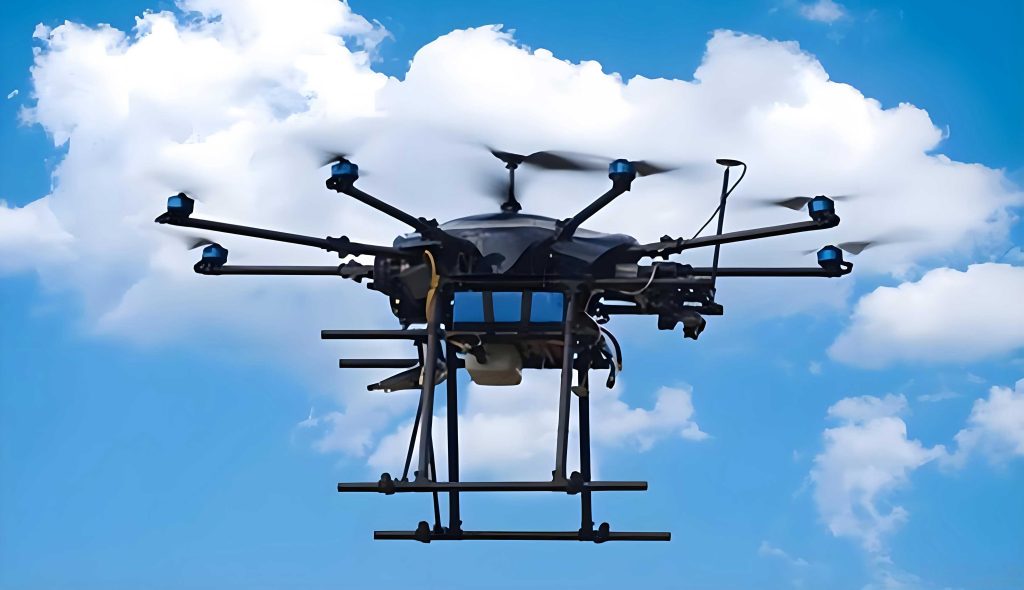
In this work, I focus on the research of cooperative navigation methods for unmanned aerial vehicles (UAVs) in complex non-line-of-sight (NLOS) environments. The presence of NLOS propagation introduces severe biases in range measurements, which significantly degrades the accuracy of conventional navigation approaches. To address this challenge, I investigate both cooperative positioning algorithms and NLOS mitigation techniques. My contributions include a distance-difference-based cooperative navigation algorithm, an NLOS identification and compensation scheme based on relative distance variation, and an improved residual weighting algorithm based on the minimum residual criterion. I validate these methods through extensive simulations under various satellite visibility conditions.
1. Introduction and Motivation
Unmanned aerial vehicles have been widely adopted in both military and civilian applications, including surveillance, search and rescue, agriculture, and traffic monitoring. However, the navigation accuracy of a single UAV is inherently constrained by its onboard sensors. Due to limitations in payload capacity, power supply, and cost, a UAV often cannot carry high-grade inertial navigation systems or multiple high-precision receivers. Cooperative navigation among a swarm of UAVs can mitigate these limitations by exploiting inter-UAV range measurements and information sharing.
In real operational scenarios, UAVs frequently operate in environments where direct line-of-sight (LOS) signals are blocked by obstacles such as buildings, trees, or terrain. These NLOS conditions introduce positive biases in range measurements because the radio signal travels along a reflected or diffracted path, which is longer than the true geometric path. The NLOS error can be much larger than the nominal measurement noise, and it severely degrades the performance of localization algorithms. Therefore, robust cooperative navigation methods that can handle complex NLOS environments are highly desirable.
2. Background and System Models
2.1 Inertial Navigation and UWB Ranging
Inertial navigation systems (INS) provide self-contained position, velocity, and attitude estimation using gyroscopes and accelerometers. The strapdown INS has become the dominant architecture in modern UAVs because it eliminates the need for a physical stable platform. The inertial measurement unit (IMU) is mounted directly on the vehicle, and a “mathematical platform” is implemented through attitude computation. The accelerometer outputs are transformed from the body frame to the navigation frame using the attitude matrix.
Ultra-wideband (UWB) technology is well suited for short-range high-precision ranging. It uses extremely short pulses over a wide frequency band, providing fine time resolution and strong resistance to multipath. I employ the symmetric double-sided two-way ranging (SDS-TWR) protocol to reduce clock drift errors. The ranging model can be expressed as:
$$ \rho_{uwb}^{i} = r^{i} + n_{uwb} + n_{NLOS}^{i} + bias \cdot r^{i} $$
where \( r^{i} \) is the true distance between the host UAV and the \( i \)-th wingman, \( n_{uwb} \) is the zero-mean Gaussian measurement noise, \( n_{NLOS}^{i} \) is the positive NLOS bias, and \( bias \) accounts for clock-related scale errors.
2.2 Extended Kalman Filter for Integrated Navigation
The extended Kalman filter (EKF) is widely used for nonlinear state estimation. For the GPS/INS tightly coupled navigation system, I define an 18-dimensional state vector:
$$ X_{c} = [\varphi_E, \varphi_N, \varphi_U, \delta v_E, \delta v_N, \delta v_U, \delta L, \delta \lambda, \delta h, \varepsilon_{bx}, \varepsilon_{by}, \varepsilon_{bz}, \varepsilon_{rx}, \varepsilon_{ry}, \varepsilon_{rz}, \nabla_x, \nabla_y, \nabla_z]^T $$
The system model is described by the equation:
$$ \dot{X}_{c} = F_{c} X_{c} + G W $$
where \( W \) is the white noise vector, \( F_{c} \) is the system matrix, and \( G \) is the noise distribution matrix. The EKF prediction and update steps are:
$$ X_{k+1|k} = f(X_{k|k}, u_k) $$
$$ P_{k+1|k} = F_k P_{k|k} F_k^T + Q_k $$
$$ X_{k+1|k+1} = X_{k+1|k} + K_{k+1} (Z_{k+1} – h(X_{k+1|k})) $$
$$ K_{k+1} = P_{k+1|k} H_{k+1}^T (H_{k+1} P_{k+1|k} H_{k+1}^T + R_{k+1})^{-1} $$
$$ P_{k+1|k+1} = (I – K_{k+1} H_{k+1}) P_{k+1|k} $$
3. Distance-Difference-Based Cooperative Navigation Algorithm
3.1 Observation Model
I consider a leader-follower architecture consisting of one host UAV and \( n \) wingmen. Each UAV is equipped with a GPS/INS tight integration system, a UWB ranging module, and a communication link. The host collects the navigation data from all wingmen and performs cooperative filtering. The relative distance between the host and the \( i \)-th wingman can be computed from their estimated positions:
$$ r^{i}_{ins} = \sqrt{(x – x_i)^2 + (y – y_i)^2 + (z – z_i)^2} $$
Linearizing this expression around the host’s true position \( (x,y,z) \) yields:
$$ r^{i}_{ins} \approx r^{i}_{0} + e_{i1} \delta x + e_{i2} \delta y + e_{i3} \delta z $$
where
$$ e_{i1} = \frac{x – x_i}{r^{i}_{0}}, \quad e_{i2} = \frac{y – y_i}{r^{i}_{0}}, \quad e_{i3} = \frac{z – z_i}{r^{i}_{0}} $$
The UWB measured distance is:
$$ \rho_{uwb}^{i} = r^{i}_{0} + n_{uwb} + n_{NLOS}^{i} + bias $$
Taking the difference between the INS-derived distance and the UWB measurement as the observation:
$$ \delta \rho^{i} = r^{i}_{ins} – \rho_{uwb}^{i} = e_{i1} \delta x + e_{i2} \delta y + e_{i3} \delta z – v^{i} $$
where \( v^{i} \) combines the measurement noise, NLOS bias, and clock bias. For \( n \) wingmen, the vectorized observation equation is:
$$ \delta \boldsymbol{\rho} = \boldsymbol{H}_{\rho} \boldsymbol{X} + \boldsymbol{V} $$
where \( \boldsymbol{H}_{\rho} \) is the observation matrix containing the directional cosines \( e_{ij} \). This observation is then fed into the EKF described in Section 2.2.
3.2 Compensation for Wingman Position Uncertainty
The wingman positions used to compute \( r^{i}_{ins} \) are themselves estimated and thus contain errors. To account for this uncertainty, I model the effect of wingman position error on the range observation. Let \( \hat{x}_b \) be the estimated position of a wingman and \( P_b \) its covariance. The variance contribution from wingman position uncertainty is:
$$ R_{b} = \boldsymbol{H}_{b} P_b \boldsymbol{H}_{b}^T $$
where \( \boldsymbol{H}_{b} \) is the Jacobian of the range function with respect to the wingman position. This term is added to the measurement noise covariance matrix \( R \) in the EKF, thereby improving the filter consistency and preventing overconfident estimates.
4. NLOS Identification and Compensation Using Relative Distance Variation
4.1 NLOS Identification
I propose a two-stage NLOS identification algorithm based on the variation of inter-UAV distances. In the first stage, the difference between consecutive UWB distance measurements is computed. Let \( M \) be the number of ranging updates in a unit time interval \( \Delta t \). The median of the absolute differences is denoted as \( \Delta D \). Since the maximum relative speed between two UAVs is \( v_{max} \), the maximum expected change in distance over \( \Delta t \) is \( 2 v_{max} \Delta t \). Accounting for measurement noise and inertial sensor drift, I set the threshold:
$$ \Theta = 2 v_{max} \Delta t + n_{uwb} + n_{IMU} $$
If \( \Delta D > \Theta \), the link is declared NLOS. Otherwise, a second test is performed using the standard deviation of the smoothed ranging measurements. Applying a Savitzky-Golay filter to obtain the smoothed range \( \hat{v}(x) \), the standard deviation is:
$$ \sigma = \sqrt{ \frac{1}{M} \sum_{m=0}^{M-1} ( \hat{v}(x_m) – u(x_m) )^2 } $$
If \( \sigma > \sigma_{LOS} \), where \( \sigma_{LOS} \) is the standard deviation measured under LOS conditions, the link is classified as NLOS. This two-stage process reduces false alarms while maintaining high detection probability.
4.2 NLOS Compensation
For links identified as NLOS, the contaminated UWB range is replaced by a reconstructed value. I combine two sources to reconstruct the measurement:
1. The distance computed from the current INS outputs of the host and wingman, denoted as \( D_{INS} \).
2. The distance predicted from the previous EKF posterior state and the current inertial displacement, denoted as \( D_{simu} \).
The reconstructed distance is:
$$ D_{real} = \alpha D_{INS} + (1 – \alpha) D_{simu} $$
The weight \( \alpha \) is selected based on the number of visible GPS satellites. When more satellites are available, the EKF posterior is more reliable, so \( D_{simu} \) gets a higher weight. Conversely, in degraded GPS conditions, the INS short-term output is more trustworthy, so \( D_{INS} \) receives a higher weight. This adaptive weighting improves robustness across different environments.
4.3 Algorithm Flow
The overall processing flow is summarized as follows:
| Step | Operation |
|---|---|
| 1 | Each UAV performs GPS/INS tight integration to obtain a preliminary position. |
| 2 | The host obtains UWB range measurements to all wingmen. |
| 3 | NLOS identification is applied to each link using the two-stage detection. |
| 4 | For NLOS links, the range is reconstructed using the adaptive weighting formula. |
| 5 | The corrected ranges are used in the distance-difference EKF to obtain the final host position. |
5. Improved Residual Weighting Algorithm
5.1 Trilateration in 3D Space
To estimate the host position from three range measurements, I use a 3D trilateration method. Given three wingmen at positions \( (x_i,y_i,z_i), i=1,2,3 \), the host position \( (x,y,z) \) satisfies:
$$ (x – x_i)^2 + (y – y_i)^2 + (z – z_i)^2 = d_i^2 $$
By subtracting the first equation from the other two and using a coordinate transformation, the solution can be obtained in closed form. The position estimate is then transformed back to the original coordinate frame.
5.2 Classic RWGH and LCC-RWGH Algorithms
The residual weighting (RWGH) algorithm forms all combinations of three base stations, computes a position estimate for each combination, and assigns a weight based on the inverse of the residual. The final estimate is the weighted sum:
$$ \hat{X} = \frac{ \sum_{k} \frac{X_k}{R_k} }{ \sum_{k} \frac{1}{R_k} } $$
where \( R_k \) is the normalized residual of the \( k \)-th combination. The LCC-RWGH algorithm reduces computational complexity by iteratively selecting the subset with the smallest residual and adding one sensor at a time.
5.3 Proposed Improved RWGH Algorithm
My improved algorithm follows the minimum residual criterion to select progressively larger subsets. The steps are:
| Step | Description |
|---|---|
| 1 | Let \( n \) be the total number of wingmen. Generate all groups of 3 wingmen. |
| 2 | For each group, compute the 3D trilateration position and the residual. |
| 3 | Select the group with the minimum residual. Record its size \( i=3 \), position \( X_3 \), and residual \( Res_3 \). |
| 4 | From the remaining wingmen, add one wingman to the selected group. Compute all possible \( (i+1) \)-sized groups and select the one with the minimum residual. Record \( X_{i+1} \) and \( Res_{i+1} \). |
| 5 | Repeat Step 4 until the group size reaches \( n \). |
| 6 | Compute the final position as a weighted sum of all recorded estimates. |
The weighting function is chosen as the inverse of the residual raised to a power \( p \):
$$ h_k = \frac{1}{Res_k^{p}} $$
After simulation experiments, I found that \( p=10 \) provides a good balance between suppressing NLOS influence and numerical stability. The final position estimate is:
$$ \hat{X} = \frac{ \sum_{k=3}^{n} h_k X_k }{ \sum_{k=3}^{n} h_k } $$
5.4 Integration with Cooperative Navigation
The corrected ranges obtained from the improved RWGH algorithm are then fed into the EKF-based cooperative navigation framework. This two-step approach—first correcting the ranges, then filtering—provides an effective way to mitigate NLOS errors without requiring prior knowledge of the NLOS distribution.
6. Simulation Results and Discussion
6.1 Simulation Setup
I simulate a UAV swarm consisting of one host and nine wingmen. All UAVs are equipped with IMU, GPS receiver, and UWB modules. The simulation parameters are listed in Table 1.
| Sensor | Parameter | Value |
|---|---|---|
| Gyroscope | Constant drift (deg/h) | 0.1 |
| White noise (deg/h) | 0.1 | |
| 1st-order Markov noise (deg/h) | 0.1 | |
| Correlation time (s) | 3600 | |
| Accelerometer | 1st-order Markov bias (g) | 0.01 |
| Correlation time (s) | 1800 | |
| GPS | Pseudorange error (m) | 3 |
| Pseudorange rate error (m/s) | 0.03 | |
| UWB | Ranging noise (m) | 0.15 |
| Clock error coefficient | 1e-3 |
The NLOS errors are simulated as positive biases uniformly distributed between 40 and 60 meters. The duration of each NLOS event is randomly set between 1 and 4 seconds. The number of wingmen simultaneously affected by NLOS varies from 2 to 7. The satellite visibility is varied among 8, 6, 3, and 1 visible satellites to model different levels of environmental harshness.
6.2 Performance with 8 Visible Satellites
In the first scenario, 8 satellites are available, but the inter-UAV links are contaminated by NLOS errors. I evaluate the reconstructed range error for selected wingmen. The RMSE values of the distance reconstruction error for wingman 1, 5, and 9 are 0.5407 m, 0.6224 m, and 0.0139 m, respectively. The improved RWGH algorithm achieves even lower reconstruction errors of 0.0139 m, 0.0149 m, and 0.0162 m, respectively. The results confirm that the proposed methods can effectively suppress NLOS biases.
| Axis | Without NLOS mitigation (m) | With NLOS mitigation (m) | Improvement factor |
|---|---|---|---|
| x | 3.5452 | 1.7928 | 1.98 |
| y | 1.8851 | 0.8197 | 2.30 |
| z | 3.0395 | 1.6938 | 1.79 |
For the improved RWGH algorithm, the results are shown in Table 3.
| Axis | Without NLOS mitigation (m) | With NLOS mitigation (m) | Improvement factor |
|---|---|---|---|
| x | 3.4987 | 1.6594 | 2.11 |
| y | 1.9022 | 0.8046 | 2.36 |
| z | 3.0457 | 1.5734 | 1.94 |
The cumulative distribution function (CDF) of the absolute positioning error becomes steeper after NLOS mitigation, indicating that the probability of large errors is greatly reduced.
6.3 Performance with 6 Visible Satellites
Reducing the satellite visibility to 6 while maintaining NLOS interference leads to larger errors for the unprocessed navigation system. My cooperative navigation algorithm still provides substantial improvements. Table 4 summarizes the RMSE results for the distance-difference EKF with NLOS compensation.
| Axis | Without NLOS mitigation (m) | With NLOS mitigation (m) | Improvement factor |
|---|---|---|---|
| x | 6.4493 | 2.0322 | 3.17 |
| y | 3.5047 | 1.0893 | 3.22 |
| z | 6.3752 | 1.9370 | 3.29 |
The improved RWGH algorithm yields the results shown in Table 5.
| Axis | Without NLOS mitigation (m) | With NLOS mitigation (m) | Improvement factor |
|---|---|---|---|
| x | 6.5392 | 1.9754 | 3.31 |
| y | 3.5512 | 1.0269 | 3.46 |
| z | 6.2852 | 1.8673 | 3.37 |
6.4 Performance with 3 Visible Satellites
With only 3 visible satellites, the GPS positioning becomes unreliable, and the unprocessed navigation errors increase significantly. My proposed algorithm still effectively improves the accuracy. The RMSE comparisons are given in Table 6 for the distance-difference EKF and Table 7 for the improved RWGH algorithm.
| Axis | Without NLOS mitigation (m) | With NLOS mitigation (m) | Improvement factor |
|---|---|---|---|
| x | 14.8751 | 3.7415 | 3.98 |
| y | 6.7481 | 1.9298 | 3.50 |
| z | 13.5110 | 3.1904 | 4.23 |
| Axis | Without NLOS mitigation (m) | With NLOS mitigation (m) | Improvement factor |
|---|---|---|---|
| x | 14.8469 | 3.5627 | 4.17 |
| y | 6.5581 | 1.7688 | 3.71 |
| z | 13.7463 | 3.1891 | 4.31 |
6.5 Performance with 1 Visible Satellite
In the most extreme case with only 1 visible satellite, the GPS is almost completely degraded. The unprocessed navigation system suffers from very large positioning errors. Nevertheless, my proposed algorithms maintain a reasonable level of accuracy, as demonstrated in Tables 8 and 9.
| Axis | Without NLOS mitigation (m) | With NLOS mitigation (m) | Improvement factor |
|---|---|---|---|
| x | 29.6469 | 6.8813 | 4.31 |
| y | 14.6995 | 3.1298 | 4.69 |
| z | 26.3210 | 6.3904 | 4.12 |
| Axis | Without NLOS mitigation (m) | With NLOS mitigation (m) | Improvement factor |
|---|---|---|---|
| x | 29.5418 | 6.7213 | 4.40 |
| y | 14.4716 | 3.0244 | 4.78 |
| z | 26.2716 | 5.8873 | 4.46 |
6.6 Discussion
The simulation results demonstrate the effectiveness of the proposed methods for unmanned aerial vehicles operating in complex NLOS environments. The distance-difference EKF algorithm leverages both INS estimates and UWB measurements in a tightly coupled framework, while the NLOS identification and compensation algorithm successfully reconstructs biased range measurements. The improved RWGH algorithm provides an alternative that does not require explicit NLOS identification and works well even when the number of LOS links is limited.
I observe that the improvement factor generally increases as the environment becomes harsher, which indicates that the proposed algorithms are particularly beneficial when conventional navigation is severely degraded. The adaptive weighting in the NLOS compensation scheme, where the weight \( \alpha \) is adjusted according to satellite visibility, contributes to the robustness. In conditions with few visible satellites, the INS provides a more reliable reference, and the corresponding weight is increased.
The improved RWGH algorithm achieves slightly better performance than the distance-difference EKF in most scenarios. This is because the RWGH algorithm effectively selects the most reliable subset of range measurements before performing the final position estimation. However, the RWGH algorithm requires trilateration with all combinations of three wingmen, which may increase computational load. In my implementation, I reduced the complexity by sequentially adding wingmen based on the minimum residual criterion, making it suitable for real-time UAV navigation.
7. Conclusion and Future Work
In this thesis, I studied cooperative navigation methods for unmanned aerial vehicles in complex NLOS environments. I proposed a distance-difference-based cooperative navigation algorithm that uses the difference between INS-derived inter-UAV distances and UWB ranging measurements as observations in an EKF. I addressed the issue of uncertain wingman positions by incorporating their covariance into the measurement noise model.
I also developed a two-stage NLOS identification algorithm based on relative distance variation and ranging standard deviation. For identified NLOS links, I reconstructed the range measurements using a weighted combination of INS outputs and the previous EKF posterior. This compensation approach avoids the loss of information that would occur if NLOS-affected measurements were simply discarded.
Furthermore, I presented an improved residual weighting algorithm that follows the minimum residual criterion to progressively build subsets of wingmen and combines the corresponding position estimates with a high-power residual weighting. Simulation results across various satellite visibility conditions confirmed that both proposed methods significantly improve the positioning accuracy of unmanned aerial vehicles in NLOS environments, with improvement factors ranging from about 1.8 to over 4.7 in different axes and scenarios.
Future work will focus on extending these methods to handle longer-duration NLOS events and complete GPS outages. I also plan to integrate visual-inertial odometry and other sensing modalities to further enhance the robustness of cooperative navigation for unmanned aerial vehicles. Additionally, machine learning techniques could be investigated for NLOS identification and ranging correction without requiring explicit threshold tuning. The ultimate goal is to develop a fully autonomous cooperative navigation framework that enables UAV swarms to operate reliably in challenging urban, forested, and indoor environments.