
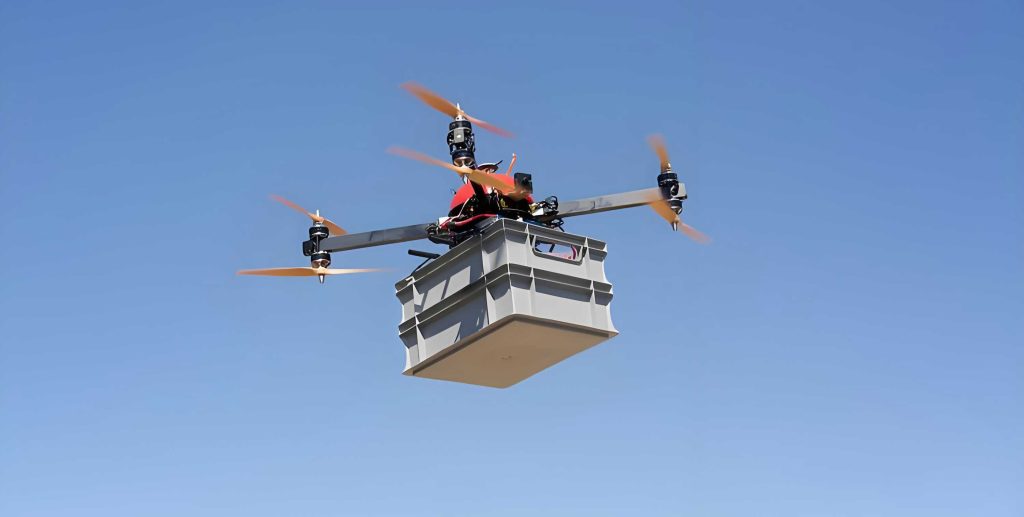
In this thesis, I focus on the challenging problem of detecting small objects in images captured by unmanned aerial vehicles. The widespread adoption of unmanned aerial vehicles in disaster relief, traffic monitoring, agricultural analysis, and film production has created an urgent need for robust and efficient perception algorithms. However, images taken from unmanned aerial vehicles differ drastically from ordinary natural images: they are captured from a top-down perspective, contain a high proportion of small objects, exhibit extreme scale variation, and are often affected by dense occlusion and inconsistent illumination. Consequently, object detectors that perform well on standard benchmarks often degrade significantly when applied to unmanned aerial vehicle imagery. To address these limitations, I propose two complementary algorithms built upon the Cascade RCNN framework. The first algorithm integrates a microscale perception module, an enhancement-location feature pyramid network, a tailored data augmentation strategy, and a balanced sampling scheme to substantially improve small-object detection accuracy. The second algorithm, named FasterDet, focuses on model efficiency by introducing a lightweight backbone, a progressive feature fusion pyramid, and a refined loss function, achieving a favorable trade-off between detection performance and computational cost. Extensive experiments on public benchmarks such as VisDrone2019 and UAVDT demonstrate that both algorithms deliver competitive results and provide practical solutions for unmanned aerial vehicles based perception systems.
1. Introduction
Object detection is one of the most fundamental and influential tasks in computer vision. It aims at identifying and localizing instances of semantic categories in images or videos. With the rapid advancement of deep learning, object detection has achieved remarkable success in many fields, including autonomous driving, surveillance, face recognition, and scene understanding. However, most existing detectors are designed for images captured by handheld cameras or fixed cameras, where objects occupy a relatively large portion of the image. In contrast, images obtained by unmanned aerial vehicles introduce a new set of challenges. Because unmanned aerial vehicles usually fly at high altitudes and use wide-angle lenses, objects such as pedestrians, vehicles, and bicycles often appear very small, sometimes only a few pixels in size. This makes feature extraction extremely difficult, especially when the objects are densely packed or partially occluded.
Small object detection in unmanned aerial vehicle imagery is particularly important for real-world applications. For example, in disaster response, unmanned aerial vehicles need to locate survivors or supplies in a wide area quickly; in traffic monitoring, they must identify vehicles and pedestrians from a high vantage point; in precision agriculture, they have to detect small crops or pests. Failing to detect these small objects can lead to severe consequences. Therefore, designing accurate and efficient detection algorithms specifically for unmanned aerial vehicle imagery is both necessary and valuable.
The primary challenges of small-object detection in unmanned aerial vehicle images can be summarized as follows. First, small objects occupy very few pixels, often less than 32×32, which means they carry limited appearance information. Second, the scale variation of the same category can be extremely large; a car in one part of the image may be dozens of times larger than a car in another part. Third, the background in aerial images is often cluttered, with buildings, roads, trees, and shadows that can easily interfere with the detector. Fourth, the imbalance between foreground and background samples, as well as between easy and hard samples, is exacerbated by the large number of small objects. Finally, the computational resources on unmanned aerial vehicles are usually limited, so models must not be excessively heavy.
In this work, I adopt Cascade RCNN as the baseline because its cascaded detection heads provide a natural way to improve localization quality. I then introduce several novel components that target the aforementioned challenges. The main contributions of this thesis are:
- A microscale perception (MSP) module that replaces standard 3×3 convolutions in the backbone. It uses two weighted deformable dilated convolution branches with different dilation rates and a learned switch to adaptively adjust the receptive field, allowing the network to extract features from objects of different scales and shapes.
- An enhancement-location feature pyramid network (E-LFPN) that aggregates all pyramid levels to obtain balanced semantic information, refines the aggregated features, and then enhances each level’s original features. It also introduces a bottom-up path to exploit precise localization information from low-level features.
- A novel data augmentation method called Cropmix that splits an image into four equal parts, enlarges each part back to the original size, and randomly recombines the enlarged parts. This operation increases the number of small-object samples and improves the model’s ability to perceive small objects.
- A balanced training strategy that combines Focal Loss with a category-aware sample extraction mechanism. This strategy mitigates both easy/hard sample imbalance and the long-tail distribution problem across categories.
- A lightweight algorithm FasterDet that replaces the backbone with a novel Faster GhostNet based on partial convolution, introduces a progressive cascade fusion feature pyramid, and adopts VariFocal Loss to reduce missed detections while preserving high efficiency.
2. Related Work
2.1 Deep Learning Object Detectors
Modern object detection methods can be broadly divided into two categories: two-stage detectors and one-stage detectors. Two-stage detectors, such as RCNN, Fast RCNN, Faster RCNN, and Mask RCNN, first generate a set of region proposals and then classify and refine them. These methods generally achieve higher accuracy but are slower than one-stage methods. One-stage detectors, such as YOLO, SSD, and RetinaNet, directly predict object categories and bounding boxes from predefined anchors or grid positions. They are faster and more suitable for real-time applications, but often struggle with small objects due to the lack of a dedicated proposal refinement stage.
Cascade RCNN is a two-stage detector that improves the quality of detection by applying a sequence of detection heads with increasing Intersection-over-Union (IoU) thresholds. This cascaded architecture effectively addresses the mismatch between the IoU distribution of proposals and the IoU threshold used for training. In this thesis, I build upon Cascade RCNN because its multi-stage refinement is especially beneficial for small objects, where precise localization is critical.
2.2 Small Object Detection
Small object detection has received increasing attention in recent years. Several lines of research have been explored to improve detection performance for small objects.
Data augmentation: A simple yet effective approach is to increase the number of small-object instances in training. For example, Kisantal et al. proposed copying and pasting small objects into other locations. Mosaic, introduced in YOLOv4, combines four images into one to enrich the training distribution. CutMix mixes two images by cutting and pasting a region, which helps the model learn from mixed contexts. My proposed Cropmix is inspired by these methods but specifically designed for unmanned aerial vehicle images, where direct scaling and recombination of patches can amplify small-object information without introducing undesired background noise.
Multi-scale representation: Many detectors use feature pyramids to detect objects across different scales. The Feature Pyramid Network (FPN) is a classic architecture that combines low-level spatial details with high-level semantic information. Variants such as PANet add a bottom-up path to improve localization. The E-LFPN that I propose takes a different angle: it aggregates all levels to form a balanced semantic representation and then uses that representation to enhance each original level. It also includes a bottom-up branch to strengthen small-object localization.
Feature fusion: Effective feature fusion is crucial for small objects. Many recent works use attention mechanisms, non-local operations, or deformable convolutions to better capture context and adapt to shape variations. My MSP module integrates weighted deformable convolutions with dilated convolutions to adaptively sample features from objects of different shapes and sizes.
Loss functions: Focal Loss is widely used to handle the foreground-background class imbalance by down-weighting easy negatives. VariFocal Loss extends this idea by using the IoU between the predicted box and the ground truth as a soft label for positive samples, allowing the model to focus more on high-quality detections. I compare these loss functions in my proposed algorithms.
2.3 UAV Object Detection
Detecting objects in unmanned aerial vehicle imagery has become a distinct research area. Many early methods cropped the large aerial image into smaller patches or used a coarse-to-fine strategy. For example, ClusDet groups objects into clusters before detection, GLSAN uses global and local search, and CZDet applies a zoom-in mechanism. While these approaches can improve detection, they often introduce significant computational overhead and require separate inference for each patch. My approach avoids the need for explicit clustering or cropping. Instead, I modify the network architecture and training procedure to handle small objects directly.
3. Problem Analysis and Motivation
To demonstrate the challenges of unmanned aerial vehicle imagery, I analyze the behavior of a standard Cascade RCNN on the VisDrone2019 dataset. The baseline model often misses small objects and sometimes misclassifies them due to insufficient appearance information. For instance, a bicycle may be misclassified as a motorcycle, and a car may be missed entirely in dense scenes. The scale variation within the same category can be enormous, as shown by the fact that the bounding box of a car in one region can be several times larger than that of a car in another region. Additionally, the class distribution is extremely unbalanced: the most frequent class (car) has more than 140,000 instances, while the least frequent class (awning-tricycle) has only about 3,000 instances. This long-tail distribution further increases the difficulty of training a robust detector.
Motivated by these observations, I design my first algorithm to improve detection accuracy by enhancing feature extraction, feature fusion, data distribution, and learning objective. The second algorithm addresses the need for real-time performance by reducing model complexity and inference time.
4. Methodology
4.1 Overview of the Proposed Algorithms
The overall framework of my first algorithm is illustrated by the modified Cascade RCNN architecture. The input image is first fed into a Cropmix data augmentation module. Then, a backbone network with the MSP module extracts multi-level features. The E-LFPN module further processes these features to produce enhanced and well-localized feature maps. The features are passed to a Region Proposal Network (RPN), and the resulting proposals are processed by three cascade detection heads. Each head uses the balanced sampling strategy and the Focal Loss function. The final output is obtained from the last detection head.
4.2 Cropmix Data Augmentation
Cropmix is designed to increase the number of small-object instances and to improve the model’s ability to learn fine-grained details. Given an input image, I first divide it into four equal quadrants. Each quadrant is then resized back to the original image size using bilinear interpolation. This magnifies the local content and helps the network learn more detailed features from small objects. However, resizing only the quadrants would change the aspect ratio and the overall object distribution. To preserve the original image distribution and introduce diversity, I also randomly select some of the original quadrants and recombine them without overlap to form a new image. During training, both the enlarged images and the recombined images are used. When objects are cut by the quadrant boundaries, I keep the object if the truncated ratio is less than 30%, otherwise the object is discarded.
The Cropmix operation has two main benefits. First, it effectively increases the number of training samples that contain large-scale views of small objects, which helps the network learn better representations. Second, it introduces more truncated objects, mimicking realistic scenarios in unmanned aerial vehicle imagery where objects often appear at the image border. The augmentation does not require any extra inference cost because it is only applied during training.
4.3 Microscale Perception Module
Receptive field size is a critical factor in detecting objects of different scales. Standard convolutional neural networks have fixed receptive fields, making it difficult to simultaneously capture very small and moderately sized objects. To address this issue, I propose the Microscale Perception (MSP) module. The module consists of three branches: two weighted deformable dilated convolution branches and one adjust-switch branch.
Let the input feature map be \(X\). The first branch applies a weighted deformable convolution with a 3×3 kernel and dilation rate 1. The second branch uses the same structure but with dilation rate 3. These two branches are designed to capture features from different scale ranges. The weighted deformable convolution learns both a spatial offset \(\Delta p_n\) and a weight \(\Delta \omega_n\) for each sampling point, allowing the convolution kernel to adapt to the shape of the object. The operation can be written as:
\[
\text{Output}(p_0) = \sum_{p_n \in R} W(p_n) \cdot X(p_0 + p_n + \Delta p_n) \cdot \Delta \omega_n
\]
where \(R = \{(1,1),(1,0),\dots,(-1,-1)\}\) is the regular grid of a 3×3 kernel, \(W(p_n)\) is the learnable weight, and \(\Delta p_n\) and \(\Delta \omega_n\) are the learned offset and weight for point \(p_n\). For the dilated branch with rate 3, the sampling positions are expanded according to the dilation rate.
The third branch is an adjust-switch branch. It first applies a global average pooling operation to obtain a global context feature. This feature is then passed through two convolutional layers to generate a switch parameter \(R\). The parameter is a value between 0 and 1 after a sigmoid activation. The final output of the MSP module is computed as a weighted sum of the two deformable branches:
\[
\text{Output} = R \cdot \text{WDDC}_{\text{rate}=1}(X) + (1-R) \cdot \text{WDDC}_{\text{rate}=3}(X)
\]
where \(\text{WDDC}\) denotes the weighted deformable dilated convolution. The switch parameter is learned end-to-end, allowing the network to choose the appropriate receptive field for each spatial location. In the backbone, I replace all 3×3 convolutions in stages 2 to 4 of ResNet50 with the MSP module. The first stage is kept frozen to preserve low-level features and reduce training cost. This design enables the network to extract multi-scale features more effectively.
4.4 Enhancement-Location Feature Pyramid Network
Feature pyramids are essential for multi-scale detection, but the standard FPN has two drawbacks. First, top-down propagation tends to weaken the original information of each level, especially for small objects. Second, high-level semantic features are propagated to low-level features, but low-level localization information is not fully exploited. To overcome these issues, I propose the Enhancement-Location Feature Pyramid Network (E-LFPN).
Let the original FPN output features be \(\{P_2, P_3, P_4, P_5\}\). The E-LFPN first aggregates these features to obtain a balanced semantic representation. To do this, I resize each feature map to the size of \(P_3\). For \(P_2\), I apply max pooling. For \(P_4\) and \(P_5\), I apply bilinear interpolation. The aggregated feature \(P_{\text{avg}}\) is computed as:
\[
P_{\text{avg}} = \frac{1}{4} \sum_{i=2}^{5} \text{Resize}(P_i)
\]
Next, \(P_{\text{avg}}\) is refined using a simplified non-local operation, which can be expressed as:
\[
y = \frac{1}{C(x)} \sum_{\forall j} \left( e^{W_\alpha x_i^T} \cdot e^{W_\beta x_j} \right) W_g x_j
\]
This refinement emphasizes informative regions and suppresses background noise. After refinement, the enhanced feature is resized back to each original level size and added to the corresponding original feature via a residual connection. This step compensates for information loss caused by the resizing operations. The resulting enhanced features are denoted as \(\{F_2, F_3, F_4, F_5\}\).
To exploit localization information from low-level features, I add a bottom-up branch. The bottom-up branch starts with \(L_2 = F_2\). For each subsequent level, I apply a 3×3 convolution with stride 2 to reduce the spatial size, then combine it with the corresponding enhanced feature using a lateral connection. This process repeats until \(L_5\) is obtained. The final feature maps \(\{L_2, L_3, L_4, L_5\}\) are then fed into the RPN and the cascade detection heads.
4.5 Loss Function and Sampling Strategy
Standard Cascade RCNN uses cross-entropy loss for classification and smooth L1 loss for regression. The cross-entropy loss suffers from the imbalance between easy and hard samples. In unmanned aerial vehicle images, the number of easy negative samples is extremely high, causing the model to focus on trivial background patterns instead of small objects. To mitigate this, I introduce Focal Loss in the classification head. Focal Loss is defined as:
\[
FL = -\alpha_t (1 – p_t)^{\gamma} \log(p_t)
\]
where \(p_t\) is the predicted probability for the true class, \(\alpha_t\) is a class-balancing weight, and \(\gamma\) is a focusing parameter. When \(\gamma = 0\), Focal Loss reduces to cross-entropy. In my experiments, I set \(\alpha_t = 0.25\) and \(\gamma = 2\). Focal Loss reduces the loss contribution from easy samples, allowing the model to focus on hard samples such as small objects.
In addition to easy/hard imbalance, the long-tail distribution among categories is another problem. For instance, in VisDrone2019, some categories have far fewer instances than others. Random sampling may cause the model to be biased toward frequent categories. I propose a category-aware sample extraction strategy. During training, I count the number of instances of each category in a mini-batch. If the number of samples for a particular category is less than the average number, I supplement the remaining samples by selecting those with the highest confidence scores from the positive proposals of that category. This strategy ensures that each category is sufficiently represented during training, thereby alleviating the long-tail distribution issue.
4.6 Lightweight FasterDet
Although the first algorithm achieves excellent accuracy, its heavy backbone and auxiliary modules increase the number of parameters and computational cost. To make the detector more suitable for embedded platforms on unmanned aerial vehicles, I propose a lightweight variant called FasterDet. The key idea is to replace the ResNet backbone with a more efficient network while preserving detection performance.
4.7 Faster GhostNet
GhostNet is a lightweight network that uses cheap operations to generate more features from a small set of intrinsic feature maps. It has shown promise in mobile applications. However, the original GhostNet uses depthwise separable convolutions, which still incur a certain amount of memory access and computational redundancy. I propose Faster GhostNet, which uses partial convolution (PConv) instead of depthwise convolution in the Ghost module and Ghost bottleneck.
The structure of a Faster Ghost module is as follows. First, a 1×1 convolution generates a set of intrinsic feature maps with half the number of output channels. Then, a partial convolution operation is applied to a subset of the channels (e.g., 1/4 of the intrinsic channels), followed by two pointwise convolutions with batch normalization and ReLU activation. The output of the pointwise convolutions is the set of ghost feature maps. Finally, the intrinsic and ghost feature maps are concatenated to form the output. This design reduces the number of computations and the amount of memory access significantly. The memory access of a standard convolution on a feature map of height \(h\) and width \(w\) with \(C\) channels is \(h \times w \times 2C\). For partial convolution, only \(C_p = C/4\) channels are involved, so the memory access becomes \(h \times w \times 2C_p\), which is four times smaller.
The Faster Ghost bottleneck is built by stacking two Faster Ghost modules. For stride 1, the bottleneck simply deepens the network. For stride 2, a partial convolution with stride 2 is inserted between the two modules to downsample the feature map. Residual connections are added to facilitate training. Faster GhostNet is then constructed by following the same architecture as GhostNet, where the convolutional layers are replaced by Faster Ghost bottlenecks. The resulting backbone extracts four feature maps with channel dimensions 24, 40, 80, and 160, which are then fed to the neck network.
4.8 Progressive Cascade Fusion Feature Pyramid
In standard feature pyramids, high-level features pass through multiple downsampling or upsampling operations before being fused with low-level features. This can cause information loss or semantic gaps between non-adjacent layers. To address this, I propose a progressive cascade fusion feature pyramid that combines features in a sequential manner using fast normalized fusion.
The input to the neck is the set of features from Faster GhostNet: \(\{C_1, C_2, C_3, C_4\}\). The fusion process proceeds progressively. First, features \(C_1\) and \(C_2\) are fused. To align their sizes, \(C_1\) is downsampled using a Space-to-Depth (S2D) operation with scale factor 2, which rearranges spatial information into channel dimensions without loss of information. \(C_2\) is upsampled by bilinear interpolation to match \(C_1\). Both resized features are then fused using fast normalized fusion. The fusion weight for each feature is determined by a learnable parameter \(\omega_i\) after a ReLU activation and batch normalization. The fused feature is computed as:
\[
C_{\text{new}} = \frac{\omega_1 \cdot C_1 + \omega_2 \cdot C_2}{\omega_1 + \omega_2 + \epsilon}
\]
where \(\epsilon = 0.0001\) is a small constant to avoid division by zero. This fast normalized fusion is more efficient than softmax and yields comparable or better results.
Next, the third feature \(C_3\) is integrated. Each of the already fused features is resized to the size of \(C_3\) using the appropriate S2D or bilinear interpolation, and then fused with \(C_3\) progressively. Finally, the fourth feature \(C_4\) is integrated in a similar manner. This progressive fusion strategy ensures that non-adjacent layers are connected directly, reducing the semantic gap and preventing the loss of small-object information. The resulting feature maps \(\{F_1, F_2, F_3, F_4\}\) contain rich semantic information from high-level layers and precise localization information from low-level layers.
4.9 VariFocal Loss for FasterDet
Although Focal Loss improves the handling of class imbalance, it treats all positive samples equally. In practice, some positive samples have higher IoU with the ground truth than others, and thus provide more reliable supervision. VariFocal Loss introduces a soft weighting for positive samples based on their IoU. The loss is defined as:
\[
\text{VFL} = \begin{cases}
– \alpha \cdot q \cdot \left( q \log(p) + (1 – q) \log(1 – p) \right), & \text{if } q > 0 \\
– \beta \cdot p^{\gamma} \cdot \log(1 – p), & \text{if } q = 0
\end{cases}
\]
where \(p\) is the predicted class probability, \(q\) is the IoU between the predicted box and the ground truth for positive samples, and for negative samples \(q = 0\). The hyperparameters \(\alpha\), \(\beta\), and \(\gamma\) control the loss weighting. In my experiments, I set \(\alpha = 0.75\) and \(\gamma = 2\). VariFocal Loss gives more weight to high-quality positive samples, which encourages the network to produce more precise bounding boxes, especially for small objects that are easily missed. It also down-weights easy negatives, similar to Focal Loss but with a different form.
5. Experiments and Analysis
5.1 Datasets and Evaluation Metrics
I evaluate the proposed algorithms on two public unmanned aerial vehicle datasets: VisDrone2019 and UAVDT.
VisDrone2019 contains 10,209 images with 12 categories. More than 380,000 annotated instances are provided. Approximately 89% of the objects are smaller than 32×32 pixels, making it a challenging benchmark for small-object detection. I exclude the “ignored” and “other” categories, leaving 10 categories for detection: pedestrian, people, bicycle, car, van, truck, tricycle, awning-tricycle, bus, and motor. The dataset is split into 6,471 training images, 3,190 test images, and 548 validation images. Since the test set annotations are not publicly available, I report results on the validation set, following common practice.
UAVDT contains about 10 hours of video captured by unmanned aerial vehicles in various traffic scenarios. The detection task is split into 23,258 training images and 15,069 test images with resolution 1080×540. The categories are car, truck, and bus.
For evaluation, I use the COCO-style mean Average Precision (mAP), mAP50, and mAP75 metrics. mAP is averaged over multiple IoU thresholds from 0.5 to 0.95 in steps of 0.05. mAP50 and mAP75 correspond to a single IoU threshold of 0.5 and 0.75, respectively.
5.2 Implementation Details
All models are implemented in PyTorch with the MMDetection toolbox. The backbone is initialized with ImageNet pre-trained weights. I adopt the 2× training schedule with 24 epochs. The optimizer is Stochastic Gradient Descent (SGD) with momentum 0.9 and weight decay 0.0001. The initial learning rate is 0.05, and is decayed by a factor of 10 at the 16th and 22nd epochs. The batch size per GPU is 2, and the number of workers is 4. Mixed-precision training (FP16) is enabled to save GPU memory. All experiments are performed on two NVIDIA GeForce GTX 1080Ti GPUs. The input images are resized to 1200×800.
5.3 Quantitative Results on VisDrone2019
Table 1 presents the comparison between my proposed algorithm (denoted as “Ours”) and various state-of-the-art detectors on the VisDrone2019 validation set. The best results are highlighted in bold. The algorithm achieves an mAP of 0.359, an mAP50 of 0.585, and an mAP75 of 0.376, outperforming all compared methods by a clear margin.
| Method | Source | mAP | mAP50 | mAP75 |
|---|---|---|---|---|
| cascadercnn+nwd* | arXiv | 0.250 | 0.434 | 0.252 |
| EdgeYOLO | arXiv | 0.264 | 0.448 | 0.262 |
| ClusDet | ICCV | 0.267 | 0.506 | 0.244 |
| QueryDet | CVPR | 0.283 | 0.481 | 0.288 |
| CEASC | CVPR | 0.287 | 0.507 | 0.284 |
| GLSAN | TIP | 0.307 | 0.554 | 0.300 |
| CZDet | CVPR | 0.322 | 0.583 | 0.262 |
| CRENet | ECCVW | 0.334 | 0.543 | 0.335 |
| Ours | – | 0.359 | 0.585 | 0.376 |
Table 1: Quantitative comparison of different methods on VisDrone2019 validation set.
Compared to the baseline Cascade RCNN, my algorithm improves mAP by 14.2 percentage points, mAP50 by 20.8 points, and mAP75 by 15.6 points. This substantial improvement is attributed to the combination of Cropmix, MSP, E-LFPN, and the balanced sampling strategy.
5.4 Quantitative Results on UAVDT
Table 2 reports the results on the UAVDT dataset. My algorithm achieves an mAP of 0.206, mAP50 of 0.312, and mAP75 of 0.209, outperforming all previously published methods that I compare with.
| Method | Source | mAP | mAP50 | mAP75 |
|---|---|---|---|---|
| Baseline | CVPR | 0.103 | 0.231 | 0.094 |
| ClusDet | ICCV | 0.137 | 0.265 | 0.125 |
| CEASC | CVPR | 0.171 | 0.309 | 0.178 |
| GLSAN | TIP | 0.197 | 0.305 | 0.217 |
| Ours | – | 0.206 | 0.312 | 0.209 |
Table 2: Quantitative comparison of different methods on UAVDT test set.
These results demonstrate that the proposed algorithm generalizes well to different unmanned aerial vehicle datasets and consistently improves detection accuracy.
5.5 Per-Class Results on VisDrone2019
To further investigate the performance on different categories, Table 3 compares the per-class AP of my algorithm with other detectors. The proposed method achieves the highest AP on nearly all categories, especially on small and frequently occluded objects such as pedestrian, people, bicycle, and motor.
| Method | mAP | car | pedestrian | tricycle | motor | people | van | bus | bicycle | awning-tricycle | truck |
|---|---|---|---|---|---|---|---|---|---|---|---|
| Retinanet | 0.159 | 0.458 | 0.124 | 0.083 | 0.106 | 0.050 | 0.243 | 0.281 | 0.034 | 0.043 | 0.171 |
| FCOS | 0.175 | 0.487 | 0.166 | 0.094 | 0.090 | 0.073 | 0.258 | 0.312 | 0.037 | 0.046 | 0.190 |
| ATSS | 0.204 | 0.513 | 0.183 | 0.141 | 0.161 | 0.060 | 0.296 | 0.319 | 0.078 | 0.073 | 0.212 |
| FasterRCNN | 0.211 | 0.496 | 0.181 | 0.143 | 0.176 | 0.109 | 0.300 | 0.326 | 0.079 | 0.073 | 0.223 |
| CascadeRCNN | 0.217 | 0.509 | 0.182 | 0.149 | 0.171 | 0.101 | 0.311 | 0.364 | 0.077 | 0.072 | 0.238 |
| DHRCNN | 0.224 | 0.510 | 0.190 | 0.161 | 0.185 | 0.124 | 0.311 | 0.363 | 0.089 | 0.068 | 0.239 |
| Ours | 0.359 | 0.609 | 0.302 | 0.310 | 0.326 | 0.217 | 0.448 | 0.573 | 0.223 | 0.188 | 0.399 |
Table 3: Per-class AP comparison on VisDrone2019 validation set.
The significant gains in pedestrian, bicycle, and motor categories indicate that the proposed algorithm is especially effective at detecting small, non-rigid objects that are often missed by other detectors.
5.6 Qualitative Results
Figure 1 shows a qualitative comparison between my algorithm and the baseline Cascade RCNN. The baseline detector frequently misses small objects in dense areas and sometimes misclassifies objects under low-light conditions. My algorithm detects more objects and produces more accurate bounding boxes. In particular, the proposed method correctly identifies objects that the baseline misses, such as distant cars, pedestrians, and even small bicycles. The improvement is consistent across different scenes, including high-altitude top-down views, oblique street views, and crowded areas.
I also observe that the number of detected targets by my algorithm is significantly higher. For example, in one high-altitude scene, the baseline detects 46 objects, while my algorithm detects 56 objects, reducing the missed detection rate from 28.1% to 12.5%. In another dense scene, the baseline misses more than 40% of the objects, whereas my algorithm misses only about 15%.
5.7 Ablation Studies
To assess the contribution of each component, I conduct ablation experiments on VisDrone2019. Starting from the baseline Cascade RCNN, I add components one by one. The results are reported in Table 4.
| Cropmix | MSP | E-LFPN | SBS | mAP |
|---|---|---|---|---|
| – | – | – | – | 0.217 |
| – | – | – | ✓ | 0.227 |
| – | – | ✓ | – | 0.236 |
| – | ✓ | – | – | 0.244 |
| ✓ | – | – | – | 0.280 |
| ✓ | – | ✓ | ✓ | 0.326 |
| ✓ | ✓ | – | ✓ | 0.334 |
| ✓ | ✓ | ✓ | ✓ | 0.359 |
Table 4: Ablation results on VisDrone2019. SBS denotes the sample balancing strategy.
Cropmix provides the largest individual improvement, increasing mAP from 0.217 to 0.280. This demonstrates that data augmentation is a powerful tool for improving small-object detection. The MSP module contributes an improvement of 2.7 percentage points when used alone, while E-LFPN contributes 1.9 points. When all components are combined, mAP reaches 0.359.
I also investigate the effect of placing the MSP module in different stages of ResNet50. Table 5 shows the results. Using MSP in stages 2 to 4 yields the best performance. Using it in all stages gives a slightly lower mAP, and removing the weighted deformable convolution reduces performance.
| Stage | mAP | mAP50 | mAP75 |
|---|---|---|---|
| 1~4 | 0.240 | 0.422 | 0.240 |
| 2~4 | 0.244 | 0.429 | 0.246 |
| 3~4 | 0.229 | 0.407 | 0.225 |
| 2~4 w/o WDDC | 0.234 | 0.411 | 0.233 |
Table 5: Effect of MSP placement in different stages.
For the E-LFPN, I evaluate the contribution of the enhancement and location branches. Table 6 shows that removing either branch lowers performance, confirming that both are beneficial.
| Model | mAP | mAP50 | mAP75 |
|---|---|---|---|
| E-LFPN | 0.236 | 0.411 | 0.240 |
| FPN | 0.217 | 0.377 | 0.220 |
| w/o location | 0.233 | 0.407 | 0.234 |
| w/o enhance | 0.231 | 0.403 | 0.233 |
Table 6: Ablation of E-LFPN branches.
I also compare Cropmix with other augmentation strategies. Table 7 shows that Cropmix outperforms Cutmix and individual crop or mix operations.
| Augmentation | mAP | mAP50 | mAP75 |
|---|---|---|---|
| Crop | 0.272 | 0.447 | 0.283 |
| Mix | 0.239 | 0.406 | 0.243 |
| Cutmix | 0.263 | 0.422 | 0.281 |
| Cropmix | 0.280 | 0.459 | 0.292 |
Table 7: Comparison of data augmentation methods.
Finally, I evaluate the effect of the sample balancing strategy on different components. Table 8 shows that the proposed SBS consistently improves performance over the original cross-entropy loss with random sampling.
| Component | Loss | mAP | mAP50 | mAP75 |
|---|---|---|---|---|
| Cascade RCNN | CE | 0.217 | 0.377 | 0.220 |
| Cascade RCNN | FL+SBS | 0.224 | 0.386 | 0.227 |
| Cropmix | CE | 0.280 | 0.459 | 0.292 |
| Cropmix | FL+SBS | 0.300 | 0.484 | 0.320 |
| MSP | CE | 0.244 | 0.429 | 0.246 |
| MSP | FL+SBS | 0.254 | 0.438 | 0.256 |
| E-LFPN | CE | 0.236 | 0.410 | 0.240 |
| E-LFPN | FL+SBS | 0.252 | 0.434 | 0.257 |
Table 8: Effect of sample balancing strategy on different components.
5.8 Computational Cost Analysis
To understand the trade-off between accuracy and efficiency, I compare the computational cost of the baseline, my first algorithm (V1), and FasterDet in Table 9.
| Model | FPS (img/s) | GFLOPs | Params (M) |
|---|---|---|---|
| Cascade RCNN | 9.5 | 224.85 | 68.95 |
| V1 | 2.2 | 174.31 | 87.63 |
| FasterDet | 5.4 | 202.87 | 71.43 |
Table 9: Efficiency comparison.
FasterDet achieves a frame rate of 5.4 img/s, which is more than double the speed of V1, while maintaining only a small decrease in accuracy. The parameter count is reduced by about 16 million compared to V1. This demonstrates the effectiveness of the lightweight backbone and the progressive fusion module.
5.9 Ablation of FasterDet
Table 10 presents the ablation study of FasterDet. The baseline is Cascade RCNN with Cropmix augmentation (mAP 0.280). Adding Faster GhostNet improves mAP to 0.305, CascadeFusionFPN to 0.314, and VariFocal Loss to 0.329. Combining all components yields 0.347.
| Faster GhostNet | CascadeFusionFPN | VariFocal Loss | mAP |
|---|---|---|---|
| – | – | – | 0.280 |
| ✓ | – | – | 0.305 |
| – | ✓ | – | 0.314 |
| – | – | ✓ | 0.329 |
| ✓ | ✓ | – | 0.335 |
| ✓ | ✓ | ✓ | 0.347 |
Table 10: Ablation results of FasterDet on VisDrone2019.
Table 11 compares the backbone efficiency between the ResNet50+MSP architecture from V1 and the proposed Faster GhostNet. Faster GhostNet nearly doubles the frame rate (from 3.0 to 6.4 img/s) while reducing the number of parameters from 83.82M to 63.86M.
| Backbone | FPS (img/s) | GFLOPs | Params (M) |
|---|---|---|---|
| ResNet50+MSP | 3.0 | 150.52 | 83.82 |
| Faster GhostNet | 6.4 | 173.31 | 63.86 |
Table 11: Backbone efficiency comparison.
I also compare different fusion methods in the progressive feature pyramid. As shown in Table 12, fast normalized fusion outperforms both concatenation and summation.
| Fusion Method | mAP | mAP50 | mAP75 |
|---|---|---|---|
| Concat | 0.342 | 0.558 | 0.343 |
| Sum | 0.338 | 0.551 | 0.336 |
| Fast Normalized Fusion | 0.347 | 0.562 | 0.351 |
Table 12: Comparison of feature fusion methods.
5.10 Visualization of Feature Maps
To further analyze the effectiveness of the proposed modules, I visualize intermediate feature maps. The visualizations show that the MSP module produces sharper and more focused features around small objects. The E-LFPN and CascadeFusionFPN both preserve target information better than the original FPN across different levels. In particular, the bottom-up path in E-LFPN keeps strong activation at low-level features, which is crucial for localization. The progressive cascade fusion in FasterDet reduces background noise and maintains independent target responses even in dense regions.
6. Conclusion and Future Work
In this thesis, I have presented a comprehensive study on small-object detection in unmanned aerial vehicle imagery using improved Cascade RCNN models. I first proposed an accurate detector that integrates a microscale perception module, an enhancement-location feature pyramid, a novel Cropmix data augmentation method, and a balanced sampling strategy. Extensive experiments on two public datasets demonstrate that the proposed method achieves state-of-the-art performance, significantly outperforming many existing detectors. Then, to address the practical need for lightweight and efficient models, I introduced FasterDet, which leverages a partial-convolution-based Faster GhostNet, a progressive cascade fusion feature pyramid, and VariFocal Loss. FasterDet more than doubles the inference speed of the first algorithm while maintaining only a small accuracy drop, making it more suitable for embedded unmanned aerial vehicle platforms.
Despite the promising results, there is still room for improvement. Future work may explore more advanced training strategies such as knowledge distillation to transfer the accuracy of the heavy model to the lightweight model. Additionally, I plan to investigate the use of transformer-based backbones for small-object detection in unmanned aerial vehicle imagery, as their global attention mechanisms may provide better context modeling. Another direction is to develop unsupervised or semi-supervised methods to reduce the reliance on expensive manual annotations. Finally, deploying the models on real unmanned aerial vehicles and testing them in end-to-end navigation and detection pipelines will be an important step toward practical applications.