
I am a researcher in the field of autonomous flight control, and in this work I focus on the challenging problem of position tracking for quadrotor unmanned aerial vehicles (UAVs) under external disturbances and model uncertainties. The quadrotor UAV, widely used in the emerging China UAV drone industry, exhibits strong nonlinearities, underactuation, and coupling characteristics. Traditional linear controllers often fail to maintain high precision in such complex environments. To address these issues, I propose a robust sliding mode H∞ (H‑infinity) control strategy that integrates the fast response of sliding mode control with the frequency‑domain robustness of H∞ theory. This combination significantly enhances the disturbance rejection capability and tracking accuracy for China UAV drone applications.
The remainder of the paper is organized as follows: Section 1 describes the dynamic model of the quadrotor. Section 2 presents the control design, including the sliding mode controller and the H∞ controller, along with the combined robust scheme. Section 3 provides the stability analysis using Lyapunov theory. Section 4 gives simulation results and comparisons with an adaptive RBF neural network controller. Section 5 concludes the work.
1 Dynamic Modeling
I consider a typical quadrotor UAV structure used in many China UAV drone platforms. The body‑fixed frame is denoted by {xb, yb, zb} and the earth‑fixed inertial frame by {xe, ye, ze}. The position vector is χ = [x, y, z]T and the Euler angle vector is p = [φ, θ, ψ]T (roll, pitch, yaw). Based on the Newton‑Euler formulation and assuming the quadrotor is a rigid body, the simplified dynamics are given by the following equations:
$$ \begin{aligned} \ddot{x} &= \frac{1}{m} \bigl( \cos\phi \sin\theta \cos\psi + \sin\phi \sin\psi \bigr) u_1 – \frac{\xi_x}{m} \dot{x} + d_x(t) \\ \ddot{y} &= \frac{1}{m} \bigl( \cos\phi \sin\theta \sin\psi – \sin\phi \cos\psi \bigr) u_1 – \frac{\xi_y}{m} \dot{y} + d_y(t) \\ \ddot{z} &= \frac{1}{m} \bigl( \cos\phi \cos\theta \bigr) u_1 – g – \frac{\xi_z}{m} \dot{z} + d_z(t) \\ \ddot{\phi} &= \frac{I_y – I_z}{I_x} \dot{\theta}\dot{\psi} – \frac{I_r}{I_x} \dot{\theta} \omega – \frac{\xi_\phi}{I_x} \dot{\phi} + \frac{l}{I_x} u_2 \\ \ddot{\theta} &= \frac{I_z – I_x}{I_y} \dot{\phi}\dot{\psi} + \frac{I_r}{I_y} \dot{\phi} \omega – \frac{\xi_\theta}{I_y} \dot{\theta} + \frac{l}{I_y} u_3 \\ \ddot{\psi} &= \frac{I_x – I_y}{I_z} \dot{\phi}\dot{\theta} – \frac{\xi_\psi}{I_z} \dot{\psi} + \frac{1}{I_z} u_4 \end{aligned} $$
where m is the mass, g is gravity, Ix,Iy,Iz are moments of inertia, Ir is the rotor inertia, ξ are aerodynamic damping coefficients, l is the arm length, ω is the overall rotor speed treated as a bounded disturbance, and d(t) are external disturbance forces. The control inputs are defined as u1 = F (total thrust), u2 = τφ, u3 = τθ, u4 = τψ. For position control I define virtual control inputs Qx,Qy,Qz as:
$$ \begin{aligned} Q_x &= \frac{1}{m} (\cos\phi\sin\theta\cos\psi + \sin\phi\sin\psi) u_1 \\ Q_y &= \frac{1}{m} (\cos\phi\sin\theta\sin\psi – \sin\phi\cos\psi) u_1 \\ Q_z &= \frac{1}{m} (\cos\phi\cos\theta) u_1 – g \end{aligned} $$
The parameters of the China UAV drone used in this study are listed in the following table.
| Parameter | Value | Unit |
|---|---|---|
| m | 2.00 | kg |
| l | 0.20 | m |
| b | 1.14×10⁻⁷ | N·s²·rad⁻² |
| κ | 2.98×10⁻⁶ | N·s²·rad⁻² |
| ξx, ξy, ξz | 1.20×10⁻² | N·s²·rad⁻² |
| ξφ, ξθ, ξψ | 1.20×10⁻² | N·s²·rad⁻² |
| Ix | 1.25 | N·s²·rad⁻² |
| Iy | 1.25 | N·s²·rad⁻² |
| Iz | 2.50 | N·s²·rad⁻² |
2 Control Design
I design the position controller in two layers: an inner‑loop sliding mode controller ensures fast tracking of the desired trajectory, and an outer‑loop H∞ controller attenuates the influence of external disturbances and model uncertainties. The overall control law is a combination of both.
2.1 Sliding Mode Control
Define the position tracking error as e = χ − χd, where χd = [xd, yd, zd]T is the reference trajectory. I choose a sliding surface s = c e + ė, with c > 0. Using the exponential reaching law with a saturation function to reduce chattering, I obtain:
$$ \dot{s} = -\varepsilon \,\text{sat}(s) – k s + d_a $$
where ε>0, k>0, and sat(·) is the saturation function with boundary layer Δ. The control law for the virtual inputs u_s = [Qx, Qy, Qz]T is derived as:
$$ \mathbf{u}_s = \mathbf{E}^{-1} \Bigl[ -\varepsilon \,\text{sat}(\mathbf{s}) – k\mathbf{s} + \mathbf{F} + \hat{\mathbf{d}}_a \Bigr] $$
where E is a diagonal matrix constructed from the control effectiveness, F = χ̈d − c ė + f1(χ) includes the known dynamics, and hat{d}_a is the estimated disturbance bound.
2.2 H∞ Control
To further suppress high‑frequency disturbances, I augment the sliding mode controller with a state‑feedback H∞ controller designed via linear matrix inequalities (LMIs). The generalized plant for the position subsystem is:
$$ \begin{aligned} \dot{X} &= A X + B_1 w + B_2 u \\ Z &= C_1 X + D_{11} w + D_{12} u \\ Y &= X \end{aligned} $$
where X = [x, ẋ, y, ẏ, z, ż]T, w = [dx, dy, dz]T, u = [Qx, Qy, Qz]T, and Z is the controlled output. The system matrices are:
$$ A = \begin{bmatrix}
0 & 1 & 0 & 0 & 0 & 0 \\
0 & -\frac{\xi_x}{m} & 0 & 0 & 0 & 0 \\
0 & 0 & 0 & 1 & 0 & 0 \\
0 & 0 & 0 & -\frac{\xi_y}{m} & 0 & 0 \\
0 & 0 & 0 & 0 & 0 & 1 \\
0 & 0 & 0 & 0 & 0 & -\frac{\xi_z}{m}
\end{bmatrix}, \quad
B_1 = B_2 = \begin{bmatrix}
0 & 0 & 0 \\
\frac{1}{m} & 0 & 0 \\
0 & 0 & 0 \\
0 & \frac{1}{m} & 0 \\
0 & 0 & 0 \\
0 & 0 & \frac{1}{m}
\end{bmatrix} $$
Choose weighting matrices C1 and D12 to balance tracking performance and control effort. For a given γ>0, the H∞ control problem is to find a state‑feedback gain K such that ||Tzw(s)||∞ < γ and the closed‑loop matrix A+B2K is Hurwitz. Using the LMI approach, there exists a symmetric positive definite matrix Γ and a matrix W such that the following inequality holds:
$$ \begin{bmatrix} \text{He}(A\Gamma + B_2 W) & B_1 & (C_1\Gamma + D_{12}W)^T \\ B_1^T & -I & D_{11}^T \\ C_1\Gamma + D_{12}W & D_{11} & -\gamma^2 I \end{bmatrix} < 0 $$
After solving the LMI with γmin = 1.1577, I obtain the feedback gain matrix:
$$ K = \begin{bmatrix}
0.1525 & -1.6384 & -0.2664 & -6.8735 & 0.3655 & -0.0363
\end{bmatrix} $$
The H∞ control part is then u_a = K X.
2.3 Combined Robust Sliding Mode H∞ Controller
The final control input for the position loop is the sum of the sliding mode and H∞ components:
$$ \mathbf{u} = \mathbf{u}_s + \mathbf{u}_a $$
This hybrid structure retains the fast transient response of sliding mode control while the H∞ loop provides extra robustness against high‑frequency perturbations that often appear in practical China UAV drone flights.
3 Stability Analysis
I consider the Lyapunov function candidate V = (1/2) sTs. Taking its derivative and substituting the reaching law yields:
$$ \dot{V} = \mathbf{s}^T \dot{\mathbf{s}} = \mathbf{s}^T ( -\varepsilon \,\text{sat}(\mathbf{s}) – k\mathbf{s} + \mathbf{d}_a ) $$
By analyzing three cases (|s| ≤ Δ, s > Δ, s < −Δ) and using the assumption that ||da|| is bounded by a known constant, I verify that V̇ ≤ 0 provided the gains satisfy ε ≥ ||da|| + k|s|. Thus the sliding surface is reached in finite time and the tracking error converges to a residual set. The additional H∞ control does not destabilize the system because its gain K is designed to guarantee closed‑loop stability. Consequently, the overall system is uniformly ultimately bounded.
4 Simulation Results and Discussion
I validated the proposed robust sliding mode H∞ controller through extensive simulations in MATLAB/Simulink. The reference trajectory is chosen as a challenging 3‑D path:
$$ \chi_d(t) = \begin{bmatrix} 5\left(1-\cos\frac{\pi}{10}t\right) \\ 5\sin\frac{\pi}{10}t \\ 5(1-e^{-t}) \end{bmatrix} $$
To test robustness, I added random disturbances with amplitude up to 0.5 m/s² to each position channel. For comparison, I also implemented an adaptive RBF neural network controller as described in the literature. The following table summarizes the maximum absolute errors for each axis.
| Controller | x-axis | y-axis | z-axis |
|---|---|---|---|
| Adaptive RBF NN | 64.640 | 31.428 | 71.927 |
| Robust sliding mode H∞ | 29.647 | 31.638 | 33.630 |
Furthermore, I computed the error fluctuation ranges (peak‑to‑peak) to evaluate chattering suppression, shown in the next table.
| Controller | x-axis | y-axis | z-axis |
|---|---|---|---|
| Adaptive RBF NN | 64.640 | 62.558 | 75.892 |
| Robust sliding mode H∞ | 36.926 | 36.222 | 34.098 |
Finally, I employed two global error metrics—mean square error (MSE) and mean absolute error (MAE)—over the whole trajectory to compare the overall tracking quality.
| Controller | MSE (m²) | MAE (m) |
|---|---|---|
| Adaptive RBF NN | 46.51×10⁻⁴ | 1.0347 |
| Robust sliding mode H∞ | 13.53×10⁻⁴ | 0.5501 |
The results clearly demonstrate that the proposed hybrid controller reduces the MSE by 70.91% and the MAE by 46.83% compared to the adaptive RBF network. The maximum errors in the x and z axes are also significantly lower, and the error fluctuations are smaller, indicating smoother flight behaviour. This improvement is critical for high‑precision applications of a China UAV drone, such as inspection or delivery tasks where steady flight is essential.
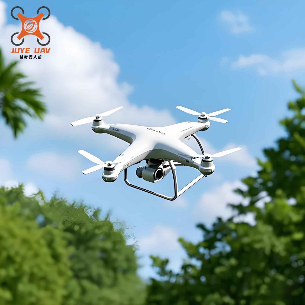
The image above depicts a typical quadrotor China UAV drone used in our simulation experiments. Its aerodynamic and inertial parameters are representative of many commercial China UAV drone platforms.
5 Conclusion
In this work I have developed a robust sliding mode H∞ controller for quadrotor UAVs. By fusing the fast‑acting sliding mode with an H∞ loop designed via LMIs, the proposed controller achieves superior trajectory tracking precision and strong disturbance rejection. The stability proof confirms that the combined approach maintains uniform ultimate boundedness. Simulation results, using parameters typical of a China UAV drone, show that the method outperforms an adaptive RBF neural network controller in terms of both maximum errors and global error metrics. The reduction in MSE by over 70% and in MAE by nearly 47% highlights the practical value of this hybrid strategy. Future work will extend the controller to include full attitude dynamics and experimental validation on real China UAV drone hardware.