
In recent years, the rapid advancement of China UAV drone technology has enabled its widespread deployment in traffic surveillance, emergency rescue, agricultural monitoring, and urban security. However, aerial images captured by UAV drones often suffer from extremely small object sizes, dense target distribution, heavy occlusion, and complex backgrounds. These challenges cause existing detectors to miss or misclassify numerous small objects. In this work, we propose an improved detection model named FPM-YOLO (Frequency-enhanced Progressive Metric-optimized YOLO) based on YOLOv8n, aiming to significantly boost small object detection performance in China UAV drone scenarios.
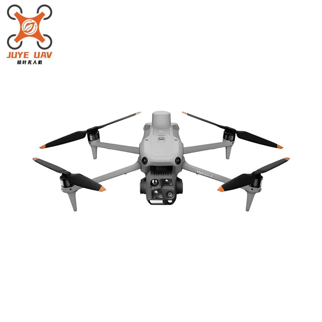
The core innovations of our method are fourfold. First, we restructure the detection head by removing the P5 head (sensitive to large objects) and introducing a high-resolution P2 head, which effectively reduces parameters while focusing computational resources on small objects. Second, we adopt a Progressive Refinement Neck (PRN) in the neck network, which reuses backbone low-level features and fuses them progressively across scales, thereby preserving spatial details for tiny targets. Third, we introduce a Gaussian Combined Distance (GCD) metric and apply it both to bounding box regression loss (combined with CIoU) and label assignment, improving matching quality and localization robustness for small objects. Fourth, we design an Edge-guided High-Frequency Enhancement Module (EHFM) that selectively amplifies contour and texture information in fused features, suppressing background noise and enhancing discriminability of small objects.
1. Methodology
1.1 Detection Layer Restructuring
The original YOLOv8 architecture performs 32× downsampling at the P5 layer. For small objects (e.g., 16×16 pixels or less), the spatial features essentially vanish after multiple stride-2 convolutions. To address this, we delete the P5 detection head and add a P2 head that operates at 4× downsampling. The resulting detection scale set becomes P2/P3/P4, which preserves high-resolution details. This change reduces the model parameter count from 3.01M to 2.01M while improving mAP50 by 3.1% in preliminary experiments (see Table 6).
1.2 Progressive Refinement Neck (PRN)
Standard PAN-FPN fuses features only once per scale, leading to gradual dilution of low-level spatial information. PRN introduces a multi-stage refinement mechanism: it reuses the backbone’s high-resolution features (especially the shallowest layers) and fuses them repeatedly via upsampling and concatenation. The neck is organized into three stages (Stage1: top-down fusion; Stage2: cross-stage re-fusion; Stage3: final refinement). This design ensures that edge and texture information is continuously preserved and combined with higher-level semantics. The parameter overhead is minimal (from 2.01M to 2.23M), yet we observe a substantial gain in recall (from 0.351 to 0.391) and mAP50 (from 0.350 to 0.409).
1.3 GCD Metric Optimization
IoU-based losses and label assignment are sensitive to small objects because a tiny shift in the prediction box can cause a drastic IoU drop. We model each bounding box as a 2D Gaussian distribution \(\mathcal{N}(\boldsymbol{\mu},\boldsymbol{\Sigma})\) with:
\[
\boldsymbol{\mu} = \begin{bmatrix} x \\ y \end{bmatrix},\quad
\boldsymbol{\Sigma} = \begin{bmatrix} \frac{w^2}{4} & 0 \\ 0 & \frac{h^2}{4} \end{bmatrix}.
\]
The GCD distance between predicted box \(B_p\) and ground truth \(B_t\) is defined as:
\[
D_{\text{gc}}^2(B_p, B_t) = \|\boldsymbol{\mu}_p – \boldsymbol{\mu}_t\|_2^2 + \operatorname{d_S}(\boldsymbol{\Sigma}_p, \boldsymbol{\Sigma}_t),
\]
where \(\operatorname{d_S}(\boldsymbol{\Sigma}_p, \boldsymbol{\Sigma}_t)\) captures scale and shape differences. We convert this to a similarity measure:
\[
\operatorname{GCD}(B_p, B_t) = \exp\bigl(-D_{\text{gc}}^2(B_p, B_t)\bigr).
\]
For bounding box regression, we use a weighted combination:
\[
L_{\text{box}} = \lambda \, L_{\text{CIoU}} + (1-\lambda) \, L_{\text{GCD}},
\]
with
\[
L_{\text{CIoU}} = 1 – \operatorname{CIoU}(B_p, B_t),\quad
L_{\text{GCD}} = 1 – \operatorname{GCD}(B_p, B_t).
\]
For label assignment, we replace the IoU term in TAL (Task-Aligned Assigner) with GCD:
\[
t_{ij} = \operatorname{GCD}(B_{p,i}, B_{t,j}),\quad
A_{ij} = s_{ij}^\alpha \cdot t_{ij}^\beta.
\]
This yields a more stable matching for small objects. Table 2 shows the effect of different \(\lambda\) values and the use of GCD in assignment. We achieve optimal mAP50 (0.325) with \(\lambda=0.5\) and GCD in assignment.
| λ | Precision | Recall | mAP50 | mAP50‑95 |
|---|---|---|---|---|
| 0+ | 0.414 | 0.326 | 0.319 | 0.181 |
| 0.3 | 0.437 | 0.321 | 0.321 | 0.183 |
| 0.4 | 0.433 | 0.322 | 0.320 | 0.183 |
| 0.4+ | 0.430 | 0.318 | 0.321 | 0.181 |
| 0.5 | 0.445 | 0.317 | 0.319 | 0.183 |
| 0.5+ | 0.430 | 0.327 | 0.325 | 0.184 |
| 0.6 | 0.435 | 0.320 | 0.320 | 0.184 |
| 0.6+ | 0.415 | 0.327 | 0.316 | 0.179 |
| 0.7 | 0.439 | 0.319 | 0.322 | 0.184 |
| 0.7+ | 0.408 | 0.330 | 0.317 | 0.180 |
| 0.8 | 0.433 | 0.314 | 0.319 | 0.184 |
We also compare GCD with EIoU and GIoU losses. The results in Table 3 show that GCD achieves the highest precision (0.445) and competitive mAP50.
| Loss | Precision | Recall | mAP50 | mAP50‑95 |
|---|---|---|---|---|
| EIoU | 0.425 | 0.326 | 0.315 | 0.182 |
| GIoU | 0.430 | 0.322 | 0.316 | 0.182 |
| GCD | 0.445 | 0.317 | 0.319 | 0.183 |
1.4 Edge‑guided High‑Frequency Enhancement Module (EHFM)
After concatenation of features from different scales, the fused feature maps contain both useful object details and background noise. EHFM separates the low-frequency component via average pooling:
\[
\mathbf{X}_{\text{lf}} = \operatorname{AvgPool}(\mathbf{X}),
\]
and obtains the high-frequency residual:
\[
\mathbf{X}_{\text{hf}} = \mathbf{X} – \mathbf{X}_{\text{lf}}.
\]
To avoid amplifying irrelevant noise, we generate an edge gate from the low-frequency component using Sobel operators (fixed kernels) followed by L1 normalization and sigmoid activation:
\[
\mathbf{E} = \sqrt{(\mathbf{X}_{\text{lf}} * K_x)^2 + (\mathbf{X}_{\text{lf}} * K_y)^2 + \epsilon},
\quad \mathbf{G} = \sigma\!\left(\frac{\mathbf{E}}{\operatorname{Mean}(\mathbf{E}) + \epsilon}\right).
\]
The enhanced output is:
\[
\mathbf{Y} = \mathbf{X} + \xi \cdot \mathbf{G} \otimes \mathbf{X}_{\text{hf}},
\]
where \(\xi\) is a learnable scalar bounded to \([0,1]\). We insert EHFM after the first concatenation in Stage1 at the P2 scale (S1-P2). Table 4 shows that this single placement yields the best mAP50‑95 (0.250) with only 4.5h training time, while adding the module at all 9 positions increases time to 5.9h without significant gain.
| Position | Precision | Recall | mAP50 | mAP50‑95 | Train time (h) |
|---|---|---|---|---|---|
| S1-P4 | 0.514 | 0.399 | 0.413 | 0.242 | 4.4 |
| S1-P3 | 0.486 | 0.414 | 0.411 | 0.241 | 4.5 |
| S1-P2 | 0.512 | 0.404 | 0.419 | 0.250 | 4.5 |
| S2-P3 | 0.495 | 0.401 | 0.409 | 0.240 | 4.5 |
| S2-P2a | 0.494 | 0.398 | 0.407 | 0.242 | 4.5 |
| S2-P2b | 0.500 | 0.405 | 0.414 | 0.242 | 4.4 |
| S3-P3 | 0.506 | 0.402 | 0.414 | 0.244 | 4.2 |
| S3-P2a | 0.504 | 0.395 | 0.407 | 0.241 | 4.5 |
| S3-P2b | 0.507 | 0.402 | 0.415 | 0.246 | 4.3 |
| All | 0.517 | 0.408 | 0.420 | 0.247 | 5.9 |
We also compare fixed Sobel vs. learnable Sobel for edge extraction. Table 5 demonstrates that fixed Sobel yields better mAP50 (0.419 vs. 0.408), as learnable kernels may diverge from stable gradient priors in cluttered backgrounds.
| Method | Precision | Recall | mAP50 | mAP50‑95 |
|---|---|---|---|---|
| Fixed Sobel | 0.512 | 0.404 | 0.419 | 0.250 |
| Learnable Sobel | 0.516 | 0.394 | 0.408 | 0.240 |
2. Experiments
2.1 Datasets and Settings
We evaluate our method on three challenging UAV datasets. The primary dataset is VisDrone2019 (collected by China UAV researchers), containing 6,471 training, 548 validation, and 1,610 test images over 10 object categories (people, pedestrians, bicycles, cars, vans, trucks, tricycles, awning tricycles, buses, motorcycles). We also test on AI-TOD (average object size 12.8 px) and UAVDT (various flight altitudes and angles) to verify generalization. All experiments use input size 640×640, batch size 8 (4 for AI-TOD due to memory), SGD optimizer with lr=0.01, momentum=0.937, weight decay=0.0005, and 200 epochs (150 for generalization).
2.2 Ablation Study
We perform a stepwise ablation on VisDrone2019 to validate each component. Results are shown in Table 6. Starting from YOLOv8n (A), we sequentially add: detection layer restructuring (B), PRN (C), GCD (D), and EHFM (F). Each addition improves performance while keeping parameters low. Full model F (FPM-YOLO) achieves 0.512 precision, 0.404 recall, 0.419 mAP50, and 0.250 mAP50‑95, with only 2.23M parameters — a 25.9% reduction compared to baseline. The GCD alone (E) still improves baseline, confirming its independent effectiveness.
| Model | Restruct. | PRN | GCD | EHFM | Params (M) | Prec. | Rec. | mAP50 | mAP50‑95 |
|---|---|---|---|---|---|---|---|---|---|
| A | 3.01 | 0.444 | 0.315 | 0.319 | 0.184 | ||||
| B | ✓ | 2.01 | 0.448 | 0.351 | 0.350 | 0.207 | |||
| C | ✓ | ✓ | 2.23 | 0.509 | 0.391 | 0.409 | 0.246 | ||
| D | ✓ | ✓ | ✓ | 2.23 | 0.526 | 0.395 | 0.416 | 0.246 | |
| E | ✓ | 3.01 | 0.430 | 0.327 | 0.325 | 0.184 | |||
| F (Ours) | ✓ | ✓ | ✓ | ✓ | 2.23 | 0.512 | 0.404 | 0.419 | 0.250 |
2.3 Comparison with State-of-the-Art
We compare FPM-YOLO against classical detectors and recent improvements on VisDrone2019. Table 7 summarizes the results. Our model achieves the highest mAP50 (41.9%) among lightweight methods, with only 2.23M parameters. It outperforms RT-DETR (r18) which uses 57M parameters, and surpasses specialized UAV detectors such as YOLO-MARS (40.9% mAP50) and MASW-YOLO (38.3% mAP50). The GFLOPs increase from 8.1 to 17.3 is a trade‑off for much higher accuracy.
| Model | mAP50 (%) | mAP50‑95 (%) | Params (M) | GFLOPs |
|---|---|---|---|---|
| SSD | 33.6 | 20.3 | 12.13 | 25.36 |
| YOLOv5n | 29.3 | 14.2 | 2.68 | 7.5 |
| YOLOv7_tiny | 34.5 | 17.5 | 6.2 | 13.1 |
| YOLOv7 | 39.6 | 22.6 | 37.2 | 104.8 |
| YOLOv8n | 31.9 | 18.4 | 3.01 | 8.1 |
| YOLOv9s | 39.4 | 23.8 | 22.1 | 61.9 |
| YOLOv10n | 31.8 | 18.2 | 2.7 | 8.2 |
| YOLOv11n | 33.7 | 20.5 | 2.58 | 6.3 |
| RT-DETR(r18) | 41.4 | 25.1 | 57 | 20 |
| LUDY-N | 35.2 | – | 2.81 | – |
| RFAG-YOLO | 38.9 | 23.1 | 5.94 | 15.7 |
| YOLO-MARS | 40.9 | 23.4 | 2.93 | – |
| REI-YOLOv8n | 36.9 | 22.3 | – | – |
| MASW-YOLO | 38.3 | 24.5 | 2.42 | 7.1 |
| FPM-YOLO | 41.9 | 25.0 | 2.23 | 17.3 |
2.4 Generalization Experiments
We further validate FPM-YOLO on AI-TOD and UAVDT datasets. Table 8 shows that on AI-TOD, our model improves mAP50 by 6.5% (from 30.8% to 37.3%) and mAP50‑95 by 3.7% compared to YOLOv8n. On UAVDT (Table 9), mAP50 increases by 1.9% (32.3% to 34.2%). These results confirm that FPM-YOLO generalizes well across different China UAV drone data sources with varying object scales and background complexities.
| Model | Precision | Recall | mAP50 (%) | mAP50‑95 (%) |
|---|---|---|---|---|
| YOLOv8n | 57.8 | 29.7 | 30.8 | 12.7 |
| FPM-YOLO | 59.7 | 36.6 | 37.3 | 16.4 |
| Model | Precision | Recall | mAP50 (%) | mAP50‑95 (%) |
|---|---|---|---|---|
| YOLOv8n | 42.5 | 30.3 | 32.3 | 19.3 |
| FPM-YOLO | 46.4 | 31.6 | 34.2 | 20.6 |
The training curves (available in our code repository) further illustrate that FPM-YOLO converges faster and achieves consistently higher mAP values compared to the baseline throughout 200 epochs.
3. Conclusion
We have presented FPM-YOLO, a novel small object detection model tailored for China UAV drone imagery. By combining detection layer restructuring, progressive refinement neck, GCD metric optimization, and edge-guided high-frequency enhancement, our method effectively addresses the issues of dense small targets, weak features, and insufficient multi-scale fusion. Extensive experiments on VisDrone2019, AI-TOD, and UAVDT datasets demonstrate that FPM-YOLO outperforms state-of-the-art lightweight detectors in both accuracy and model efficiency, with only 2.23M parameters. Future work will focus on further reducing computational overhead while maintaining detection capability, enabling real-time deployment on embedded UAV platforms.