
Unmanned aerial vehicles (UAVs) operate in highly dynamic and adverse environments, where factors such as turbulence, vibration, component aging, and deformation degrade performance over time. Among various UAV platforms, the fixed-wing UAV is widely adopted due to its long endurance, high altitude capability, large payload, and extended flight range. However, these advantages come with increased complexity and vulnerability to actuator faults, which can lead to catastrophic mission failures. Actuator faults are particularly dangerous because they directly affect control surfaces (elevons, rudders, etc.) and can manifest as partial loss of effectiveness, lock-in-place, or intermittent malfunctions. Traditional model-based fault diagnosis methods require accurate mathematical models of the nonlinear, tightly coupled fixed-wing UAV dynamics, which are often difficult to derive. Moreover, these models are sensitive to uncertainties and disturbances, limiting their diagnostic accuracy in real-world scenarios.
With the advent of big data and deep learning, data-driven approaches have shown remarkable promise for fault diagnosis without explicit system models. Among deep learning architectures, convolutional neural networks (CNNs) have demonstrated superior feature learning and representation capabilities, especially in processing time-series signals. In this work, we present a comprehensive study on applying CNNs to the fault diagnosis of fixed-wing UAV actuators. Our approach leverages raw flight data—linear accelerations, angular rates, and actuator commands—to automatically extract discriminative features that characterize various actuator degradation levels. We validate the proposed method using real flight experiments from a fixed-wing UAV under different wind conditions, and we analyze the model’s generalization ability across flights with varying environmental complexities.
The key contributions of this paper are threefold. First, we design a compact yet effective CNN architecture tailored for fixed-wing UAV fault diagnosis, comprising multiple convolutional and pooling layers followed by a fully connected layer and a softmax classifier. Second, we construct a fault injection framework that simulates eight distinct actuator efficiency loss levels (ranging from 30% to 90% effectiveness) based on a realistic actuator model. Third, through systematic cross‑flight evaluations, we uncover the critical influence of training data complexity on model generalization and provide recommendations for practical deployment. Extensive experiments demonstrate that the proposed CNN achieves over 99% classification accuracy on in‑distribution data and significant improvements on cross‑distribution scenarios when trained on more challenging flight conditions.
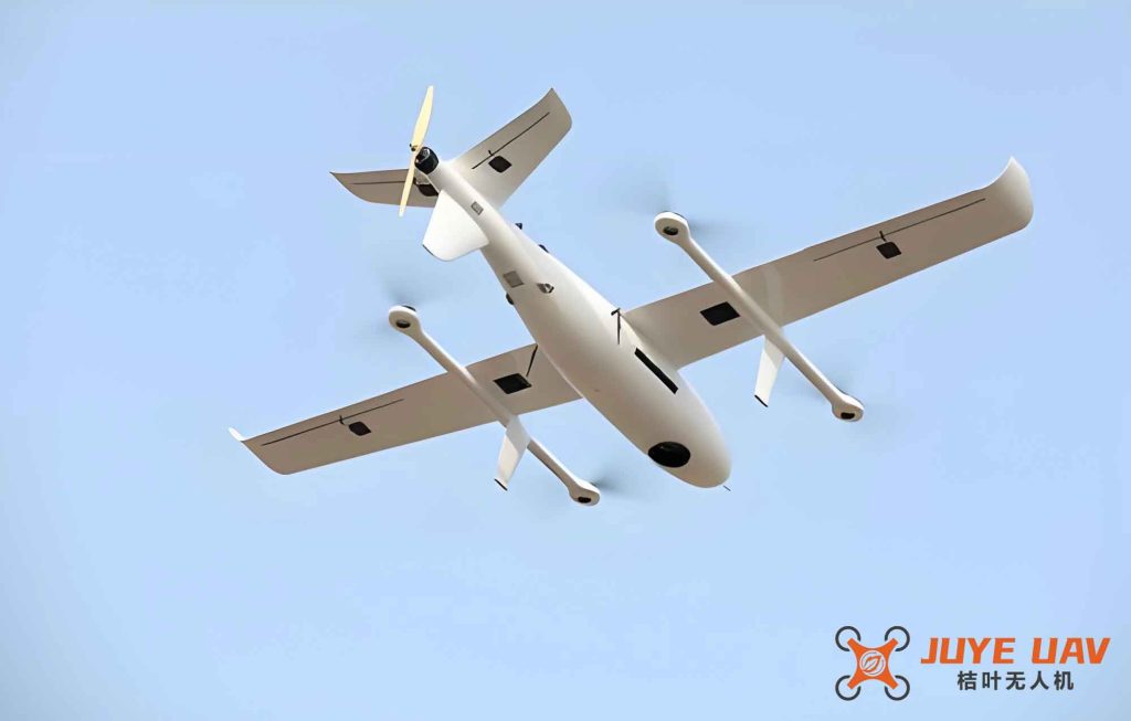
1. Problem Formulation and Actuator Fault Modeling
We consider a fixed-wing UAV equipped with two primary control surfaces: the right elevon and the left elevon. The actuator fault can be expressed by the following model:
$$
\mathbf{u}_{\text{app}} = \mathbf{D} \mathbf{u}_{\text{com}} + \mathbf{e},
$$
where \(\mathbf{u}_{\text{com}} \in \mathbb{R}^2\) is the commanded deflection from the autopilot, \(\mathbf{u}_{\text{app}} \in \mathbb{R}^2\) is the actual applied deflection, \(\mathbf{D} = \operatorname{diag}(d_1, d_2)\) is a diagonal matrix representing the efficiency factor of each actuator (with \(d_i \in [0,1]\)), and \(\mathbf{e} = [e_1, e_2]^\top\) is a bias vector. In our study, we focus on efficiency loss faults by setting the bias to zero and varying the diagonal entries. For instance, \(d_1=0.3\) indicates that the right elevon retains only 30% of its nominal effectiveness. Fault codes 0 through 8 correspond to nine distinct conditions, as summarized in the table below.
| Fault Code | Description | \(d_1\) | \(d_2\) |
|---|---|---|---|
| 0 | Nominal (no fault) | 1.0 | 1.0 |
| 1 | Right elevon efficiency 0.3 | 0.3 | 1.0 |
| 2 | Left elevon efficiency 0.9 | 1.0 | 0.9 |
| 3 | Left elevon efficiency 0.8 | 1.0 | 0.8 |
| 4 | Left elevon efficiency 0.7 | 1.0 | 0.7 |
| 5 | Left elevon efficiency 0.6 | 1.0 | 0.6 |
| 6 | Left elevon efficiency 0.5 | 1.0 | 0.5 |
| 7 | Left elevon efficiency 0.4 | 1.0 | 0.4 |
| 8 | Left elevon efficiency 0.3 | 1.0 | 0.3 |
The flight data we use originate from a real fixed-wing UAV platform (detailed specifications: wing span 1.2 m, surface area 0.28 m², mass 0.75 kg, battery capacity 30 Wh, flight time ~60 min). The aircraft performs an autonomous figure‑eight pattern under two different wind conditions: 2.5 m/s (Flight A on 21 June) and 5.0 m/s (Flight B on 23 June). During each flight, multiple fault segments are injected in sequence: three consecutive right‑elevon efficiency faults (code 1), then three consecutive left‑elevon efficiency faults (code 2 through 8), separated by nominal phases. Each fault lasts approximately one full figure‑eight loop.
2. Feature Trajectory Construction
To reduce computational cost and filter out irrelevant variations, we select eight raw measurements as the basic feature set:
$$
\mathbf{X’}(t) = \big[ a_x(t),\, a_y(t),\, a_z(t),\, \omega_x(t),\, \omega_y(t),\, \omega_z(t),\, u_{\text{com1}}(t),\, u_{\text{com2}}(t) \big]^\top,
$$
where \(a\) denotes linear acceleration, \(\omega\) angular rate, and \(u_{\text{com1}}, u_{\text{com2}}\) the commanded deflections for the two elevons. To incorporate temporal dynamics, we concatenate 20 consecutive samples (the current time instant \(t\) and the previous 19 instants). This yields a 160‑dimensional input vector \(\mathbf{X}(t)\) for the CNN:
$$
\mathbf{X}(t) = \big[ \mathbf{X’}(t-19),\; \mathbf{X’}(t-18),\; \dots,\; \mathbf{X’}(t-1),\; \mathbf{X’}(t) \big] \in \mathbb{R}^{160}.
$$
This sliding‑window approach preserves the short‑term evolution of the flight dynamics, which is crucial for distinguishing subtle efficiency changes in the actuators.
3. Convolutional Neural Network Architecture
The CNN model we design for fixed-wing UAV fault diagnosis consists of five alternating convolutional and max‑pooling layers, followed by one fully‑connected hidden layer with 100 neurons and a softmax layer for multi‑class classification. The structure is illustrated conceptually as:
Input (160×1) → Conv1 → Pool1 → Conv2 → Pool2 → Conv3 → Pool3 → Conv4 → Pool4 → Conv5 → Pool5 → FC (100) → Softmax (9 classes).
All convolutional kernels are of size \(3 \times 1\), stride \(1 \times 1\), and the same padding is applied to preserve temporal resolution. Each convolutional layer computes the following operation:
$$
y^{(l)}(i,j) = \sum_{j’=0}^{W-1} K^{(l)}_i(j’)\, x^{(l)}_r(j+j’),
$$
where \(K^{(l)}_i\) is the \(i\)-th kernel of the \(l\)-th layer, \(W=3\) is the kernel width, and \(x^{(l)}_r\) is the local region of the input feature map. After convolution, we apply the rectified linear unit (ReLU) activation:
$$
a^{(l)}(i,j) = f\big(y^{(l)}(i,j)\big) = \max\{0,\; y^{(l)}(i,j)\}.
$$
ReLU provides sparse activation and mitigates the vanishing gradient problem. For down‑sampling, we employ max‑pooling with a window size of \(2 \times 1\) and stride \(2\), defined as:
$$
p^{(l)}(i,j) = \max_{(j-1)W+1 \leq t \leq jW} \big\{ a^{(l)}(i,t) \big\}.
$$
The final fully‑connected layer concatenates the output of the last pooling layer into a vector and produces a 100‑dimensional feature representation. The softmax layer then computes the probability distribution over the nine fault categories. The loss function is the cross‑entropy between the predicted probabilities and the one‑hot encoded labels:
$$
\mathcal{L} = -\frac{1}{m} \sum_{k=1}^{m} \sum_{j=1}^{9} \mathbf{1}\{y_k = j\} \log \hat{p}_{k,j},
$$
where \(m\) is the mini‑batch size, \(y_k\) is the true label, and \(\hat{p}_{k,j}\) is the softmax output for class \(j\). Training is performed using Adam optimizer with an initial learning rate of 0.001, mini‑batch size 64, and 50 epochs. Early stopping is applied if validation loss does not improve for 10 consecutive epochs.
4. Experimental Setup
We conduct two sets of experiments to evaluate the performance of the proposed CNN for fixed-wing UAV fault diagnosis.
4.1 Data Partitioning
For the first experiment (in‑distribution evaluation), we use Flight A (21 June, wind 2.5 m/s). The recorded time series between 400 s and 2600 s is divided into training (80%) and testing (20%) sets, ensuring no temporal overlap. Each sample is labeled according to the fault code in effect at that time. The total number of test samples is 4403, with class distribution varying due to fault durations.
4.2 Cross‑Flight Generalization
For the second experiment, we assess the model’s ability to generalize to a different flight environment. Two directions are tested:
- Scenario A→B: Train on Flight A (wind 2.5 m/s) and test on Flight B (wind 5.0 m/s).
- Scenario B→A: Train on Flight B and test on Flight A.
These scenarios simulate a realistic condition where a diagnostic model trained on historical data must perform online on a new mission with potentially different environmental conditions.
4.3 Evaluation Metrics
We adopt four standard classification metrics:
- Accuracy = (correct predictions) / (total samples)
- Precision = true positives / (true positives + false positives)
- Recall = true positives / (true positives + false negatives)
- F1-score = 2 × (precision × recall) / (precision + recall)
For comparison, we also train a support vector machine (SVM) with a radial basis function kernel on the same training data. The SVM is widely used as a traditional machine‑learning baseline for fault diagnosis.
5. Results and Discussion
5.1 In‑Distribution Performance
The CNN achieves outstanding results on the test set from Flight A. Table 1 reports per‑class precision, recall, F1‑score, and overall accuracy.
| Fault Code | Precision | Recall | F1‑Score | Support |
|---|---|---|---|---|
| 0 (nominal) | 1.00 | 1.00 | 1.00 | 1382 |
| 1 (R0.3) | 1.00 | 1.00 | 1.00 | 485 |
| 2 (L0.9) | 1.00 | 1.00 | 1.00 | 295 |
| 3 (L0.8) | 1.00 | 0.99 | 0.99 | 299 |
| 4 (L0.7) | 0.99 | 0.98 | 0.98 | 299 |
| 5 (L0.6) | 0.98 | 1.00 | 0.99 | 311 |
| 6 (L0.5) | 1.00 | 1.00 | 1.00 | 306 |
| 7 (L0.4) | 1.00 | 0.99 | 1.00 | 323 |
| 8 (L0.3) | 1.00 | 1.00 | 1.00 | 703 |
| Overall | 0.99 | 0.99 | 0.99 | 4403 |
The overall accuracy is 99%, with macro‑averaged precision, recall, and F1‑score all at 1.00 (or 0.99). The CNN effectively distinguishes between similar efficiency levels (e.g., 0.9 vs. 0.8 for left elevon). In contrast, the SVM baseline achieves only 93% accuracy, as shown in Table 2.
| Fault Code | Precision | Recall | F1‑Score | Support |
|---|---|---|---|---|
| 0 (nominal) | 0.92 | 0.98 | 0.94 | 1382 |
| 1 (R0.3) | 0.98 | 0.93 | 0.95 | 485 |
| 2 (L0.9) | 0.85 | 0.70 | 0.77 | 295 |
| 3 (L0.8) | 0.87 | 0.90 | 0.88 | 299 |
| 4 (L0.7) | 0.94 | 0.90 | 0.92 | 299 |
| 5 (L0.6) | 0.89 | 0.90 | 0.90 | 311 |
| 6 (L0.5) | 0.91 | 0.89 | 0.90 | 306 |
| 7 (L0.4) | 0.95 | 0.93 | 0.94 | 323 |
| 8 (L0.3) | 0.97 | 0.98 | 0.98 | 703 |
| Overall | 0.93 | 0.90 | 0.91 | 4403 |
To further understand the CNN’s internal representations, we apply t‑distributed stochastic neighbor embedding (t‑SNE) to the 100‑dimensional features from the fully‑connected layer. The resulting 2D projection clearly separates the nine classes into distinct clusters, confirming that the network learns discriminative fault‑specific patterns.
5.2 Cross‑Flight Generalization
When we train the CNN on Flight A and test it on Flight B (scenario A→B), the performance drops significantly, as shown in Table 3. The overall accuracy is only 52%, and many classes (especially code 2 and 3) exhibit extremely low precision and recall.
| Fault Code | Precision | Recall | F1‑Score | Support |
|---|---|---|---|---|
| 0 (nominal) | 0.89 | 0.57 | 0.70 | 1649 |
| 1 (R0.3) | 0.72 | 0.62 | 0.67 | 505 |
| 2 (L0.9) | 0.10 | 0.33 | 0.15 | 144 |
| 3 (L0.8) | 0.16 | 0.38 | 0.22 | 152 |
| 4 (L0.7) | 0.39 | 0.65 | 0.49 | 264 |
| 5 (L0.6) | 0.57 | 0.41 | 0.47 | 301 |
| 6 (L0.5) | 0.56 | 0.60 | 0.58 | 310 |
| 7 (L0.4) | 0.49 | 0.45 | 0.47 | 324 |
| 8 (L0.3) | 0.79 | 0.80 | 0.80 | 752 |
| Overall | 0.52 | 0.54 | 0.51 | 4401 |
The failure is primarily due to distributional shift: Flight B experiences stronger winds (5.0 m/s vs. 2.5 m/s), resulting in more turbulent dynamics and different angular rate profiles. The CNN, trained exclusively on calm‑condition data, overfits to the specific patterns of Flight A and fails to generalize.
However, when we reverse the training and testing sets (scenario B→A), we observe a substantial improvement, as reported in Table 4. The overall accuracy rises to 66%, and most classes achieve F1‑scores above 0.5, with nominal and severe fault (code 8) exceeding 0.80.
| Fault Code | Precision | Recall | F1‑Score | Support |
|---|---|---|---|---|
| 0 (nominal) | 0.76 | 0.94 | 0.84 | 1382 |
| 1 (R0.3) | 0.71 | 0.79 | 0.74 | 485 |
| 2 (L0.9) | 0.37 | 0.06 | 0.10 | 295 |
| 3 (L0.8) | 0.66 | 0.43 | 0.52 | 299 |
| 4 (L0.7) | 0.71 | 0.55 | 0.62 | 299 |
| 5 (L0.6) | 0.66 | 0.44 | 0.53 | 311 |
| 6 (L0.5) | 0.56 | 0.72 | 0.63 | 306 |
| 7 (L0.4) | 0.66 | 0.61 | 0.63 | 323 |
| 8 (L0.3) | 0.82 | 0.91 | 0.87 | 703 |
| Overall | 0.66 | 0.61 | 0.61 | 4403 |
The improvement in scenario B→A suggests that training on more complex, high‑wind data forces the network to learn more robust, invariant features. The CNN exposed to larger variability in angular rates and accelerations becomes less sensitive to the specific dynamics of the calmer scenario. This insight is crucial for practical deployment: when designing a diagnostic system for fixed-wing UAV, one should preferentially include data from the most challenging operating conditions in the training set.
6. Discussion on Overfitting and Generalization
The cross‑flight experiment reveals a typical overfitting problem in deep learning when the training distribution is narrow. Our CNN achieves near‑perfect accuracy on the hold‑out portion of Flight A, but fails on Flight B because the model has memorized patterns that are specific to the 2.5 m/s wind regime. This is evidenced by the sharp drop in accuracy from 99% to 52% when evaluating on a different flight condition.
To mitigate overfitting, we consider two practical strategies:
- Data augmentation: Simulating additional wind speeds or injecting synthetic noise could enlarge the effective training distribution.
- Domain‑adversarial training: Incorporating a domain classifier during training encourages the feature extractor to learn domain‑invariant representations.
Nevertheless, the B→A results demonstrate that simply using more diverse real data (higher wind) can already improve robustness without additional algorithmic complexity. In production environments, collecting flight data under various weather conditions and maneuver types is recommended.
7. Real‑Time Considerations for Fixed-Wing UAV
For online fault diagnosis aboard a fixed-wing UAV, computational latency and memory footprint are critical. Our CNN model has only 5 convolutional layers (each with 3×1 kernels) and one small fully‑connected layer, resulting in approximately 50,000 trainable parameters. Inference on a single 160‑dimensional input takes less than 1 ms on a modern embedded GPU (e.g., NVIDIA Jetson Nano). The memory requirement is under 2 MB. This makes the proposed architecture suitable for real‑time deployment on resource‑constrained flight controllers.
A typical online diagnostic pipeline would involve:
- Buffering the last 20 time steps of the 8‑channel sensor stream (160 floating‑point values).
- Passing the buffer through the CNN every 20 ms (or at 50 Hz).
- Monitoring the softmax output; if the probability of any fault class exceeds a predefined threshold (e.g., 0.8), an alert is triggered.
Such a system can provide early warnings for gradual actuator degradation, enabling the autopilot to trigger corrective actions or initiate a safe landing procedure.
8. Conclusion
In this work, we have presented a comprehensive study on using convolutional neural networks for fixed-wing UAV actuator fault diagnosis. The proposed CNN architecture, with its alternating convolutional and pooling layers and a fully‑connected classifier, automatically extracts hierarchical features from raw flight data—linear accelerations, angular rates, and actuator commands. On in‑distribution data from a fixed-wing UAV flight under moderate wind, the model achieves 99% accuracy, outperforming a traditional SVM baseline by 6 percentage points.
However, when applied to a flight with stronger wind (5 m/s), the model trained solely on calm data exhibits severe performance degradation, with accuracy dropping to 52%. This overfitting issue is largely mitigated by training on the more complex high‑wind flight data first; the resulting model achieves 66% accuracy on the calm flight, demonstrating that exposure to greater environmental variability improves generalization. The key takeaway for practitioners is the importance of training data diversity: to build a reliable fixed-wing UAV fault diagnosis system, one should incorporate flight data from the most challenging operating conditions expected in the field.
Future work will explore domain‑adaptation techniques and test the CNN on a broader range of fault types (e.g., intermittent faults, sensor faults, and actuator jamming). Additionally, we plan to integrate the diagnostic module into a real‑time onboard flight computer and validate its performance in live flight experiments with injected faults. The ultimate goal is to create a robust, lightweight, and practical solution that enhances the safety and mission success rate of fixed-wing UAV operations.