
In our research, we address the critical challenge of aerial docking for fixed-wing UAVs, which is a key bottleneck in the development of chained-wing UAV systems. The wing docking process involves complex aerodynamic coupling between two UAVs in close proximity, particularly due to wingtip vortex interactions. To tackle this, we develop a comprehensive aerodynamic modeling framework based on the numerical lifting-line method and propose an optimal path planning strategy using the Dijkstra algorithm. Our work focuses on accurately capturing the aerodynamic interference during the docking maneuver and identifying a trajectory that minimizes adverse effects on lift and rolling moment. The entire study is conducted from the perspective of designing a reliable docking guidance system for fixed-wing UAVs.
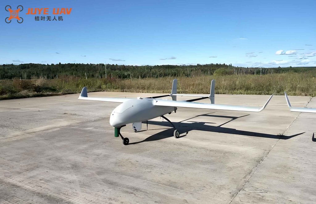
The aerodynamic modeling is built upon the generalized numerical lifting-line method, known as the G-H method. This approach extends the classical Prandtl lifting-line theory to handle arbitrary wing geometries with sweep and dihedral, enabling accurate computation of induced velocities and aerodynamic loads in multi-wing configurations. We apply this method to two identical fixed-wing UAVs approaching each other for wingtip docking. The UAV parameters are summarized in Table 1.
| Parameter | Value |
|---|---|
| Airfoil | NACA0010 |
| Weight (N) | 20 |
| Half span (m) | 2 |
| Chord length (m) | 1 |
| Fuselage length (m) | 1 |
| Vertical tail chord (m) | 0.4 |
| Vertical tail span (m) | 0.5 |
| Vertical tail sweep (°) | 20 |
| Horizontal tail chord (m) | 0.4 |
| Horizontal tail span (m) | 0.5 |
| Horizontal tail sweep (°) | 20 |
The G-H method defines the lifting-line geometry using a parametric representation along the dimensionless spanwise coordinate \( s \). The original lifting-line position vector is given by:
$$
\mathbf{r}_{LL}(s) = \mathbf{r}_{LL}(0) + \frac{b}{2} \begin{bmatrix} -\int_0^s \tan\Lambda(\sigma) d\sigma \\ \int_0^s \cos\Gamma(\sigma) d\sigma \\ \int_0^s \sin\Gamma(\sigma) d\sigma \end{bmatrix}, \quad -1 \le s \le 1
$$
where \(\Lambda(s)\) and \(\Gamma(s)\) are the local sweep and dihedral angles, and \(b\) is the total wingspan. Control points are distributed using a cosine clustering to improve convergence:
$$
s_i = \frac{1}{2}\left[1 – \cos\left(\frac{\pi}{2N} + \frac{i\pi}{N}\right)\right], \quad i=0,1,\dots,N-1
$$
To avoid curvature singularities at control points, an effective lifting-line is introduced through a Gaussian blending function:
$$
\tilde{\mathbf{r}}^i_{LL}(s) = (1 – e^{-\sigma(s-s_i)^2}) \mathbf{r}_{LL}(s) + e^{-\sigma(s-s_i)^2} \left[ \mathbf{r}_{LL}(s_i) + \left.\frac{d\mathbf{r}_{LL}}{ds}\right|_{s=s_i}(s-s_i) \right]
$$
The parameter \(\sigma\) is chosen such that the effective line has a straightness of 0.018% at a dimensionless distance \(\Delta s_b = 1\). The horseshoe vortices are placed with their bound segments along the quarter-chord line, and trailing vortices extend infinitely downstream aligned with the local velocity direction. The induced velocity at each control point is computed using the Biot-Savart law, accounting for the contributions from all vortex elements.
The aerodynamic force on each wing segment is derived from the effective section properties. For a swept wing, the effective chord, Reynolds number, and angle of attack are defined in the plane perpendicular to the lifting line. The effective angle of attack is:
$$
\alpha_{\Lambda} = \arctan\left( \frac{\mathbf{V}_{\Lambda} \cdot \mathbf{u}_{n\Lambda}}{\mathbf{V}_{\Lambda} \cdot \mathbf{u}_{a\Lambda}} \right)
$$
where \(\mathbf{V}_{\Lambda}\) is the effective velocity, and \(\mathbf{u}_{n\Lambda}\), \(\mathbf{u}_{a\Lambda}\) are the normal and axial unit vectors. The lift coefficient of a swept section can be related to the unswept airfoil data through thin-airfoil theory:
$$
\alpha_{L0\Lambda} = \frac{\alpha_{L0}}{\cos\Lambda}
$$
For small angles, the lift coefficient is linearized as:
$$
\tilde{C}_{L\Lambda}(\alpha_{\Lambda}) \approx \tilde{C}_{L,\alpha}(\alpha_{\Lambda} + \alpha_{L0} – \alpha_{L0\Lambda})
$$
The governing equation of the G-H method is derived by equating the lift from Kutta-Joukowski theorem with that from the sectional lift coefficient:
$$
\rho \Gamma_i |\mathbf{V}_{\Lambda,i} \times d\mathbf{l}_i| = \frac{1}{2} \rho V_{\Lambda,i}^2 \tilde{C}_{L\Lambda,i} \Delta S_i
$$
After linearization, the system becomes a set of linear equations for the unknown vortex strengths \(\Gamma_i\):
$$
2|\mathbf{V}_{\infty+\omega,\Lambda,i} \times d\mathbf{l}_i| \Gamma_i – V_{\infty\Lambda,i} \tilde{C}_{L,\alpha,i} \Delta S_i \sum_{j=1}^N \Gamma_j (\mathbf{v}_{ji}\cdot\mathbf{u}_{n\Lambda,i}) = V_{\infty\Lambda,i}^2 C_{L\Lambda,i}(\alpha_{\infty+\omega}) \Delta S_i
$$
For nonlinear cases, we employ Newton iteration to solve the full system. The Jacobian matrix is constructed, and the vortex strengths are updated with a relaxation factor \(\psi\):
$$
\Gamma^{k+1} = \Gamma^k + \psi \Delta \Gamma
$$
Once the circulation distribution is obtained, the total force and moment on each UAV are computed. We validated the G-H method against experimental data for a 45° swept wing with NACA0010 airfoil, and the results show excellent agreement.
Aerodynamic Database for Wing Docking
To analyze the aerodynamic interference during the docking process, we simulate two fixed-wing UAVs at the same altitude with identical angle of attack. The leader UAV maintains a steady level flight, while the follower UAV approaches from the right-rear side. We define a planar coordinate system with the origin at the final docked configuration. The relative position is parameterized by the spanwise gap \(y\) and chordwise gap \(x\) (positive when the follower is behind the leader). The simulation conditions are listed in Table 2.
| Parameter | Value |
|---|---|
| Free-stream velocity (m/s) | 10 |
| Angle of attack (°) | 2 |
| Spanwise gap (m) | 0, 0.4, 0.8, …, 4.0 |
| Chordwise gap (m) | 0, 0.4, 0.8, …, 4.0 |
Figure 1 (not shown) in the original paper illustrates two typical docking scenarios: Case 1 – spanwise approach (chordwise gap fixed at zero, varying spanwise gap), and Case 2 – chordwise approach (spanwise gap fixed at zero, varying chordwise gap). The aerodynamic forces and moments acting on the follower UAV are computed for all grid points. The results reveal significant aerodynamic coupling when the UAVs are close, with lift and rolling moment variations of up to 20% compared to isolated flight. For instance, when the follower is directly behind the leader (zero spanwise gap), the lift decreases as the chordwise gap reduces due to the downwash from the leader’s wingtip vortex. Conversely, when approaching purely in the spanwise direction, the rolling moment exhibits strong gradients near the wingtip contact point.
The complete aerodynamic database maps the lift \(L\) and rolling moment \(M\) as functions of \((x,y)\). The contour plots (not shown) indicate that the coupling effect decays rapidly with spanwise separation, but persists over longer chordwise distances. In quantitative terms, when the distance exceeds approximately four chord lengths, the interference becomes negligible. However, at close range (within one chord), the coupling is severe. These observations motivate the need for an optimized docking path that avoids high-interference regions.
Path Optimization Using Dijkstra Algorithm
We formulate the wing docking path planning as a weighted directed shortest path problem. The state space consists of discrete relative positions \((x_i, y_i)\) on a uniform grid. The follower UAV is allowed to move only towards the leader (i.e., decreasing the distance in both spanwise and chordwise directions). Thus, from each node, three possible moves are considered: left (decreasing \(y\)), forward (decreasing \(x\)), or diagonal (decreasing both). The cost associated with moving from node \(i\) to node \(j\) is defined as:
$$
G(i,j) = k_F \bar{F}_{i,j} + k_M \bar{M}_{i,j}
$$
where \(\bar{F}_{i,j}\) and \(\bar{M}_{i,j}\) are normalized aerodynamic load and moment penalties averaged over the transition. The normalization is performed with respect to the values at a reference position (\(x=10\) m, \(y=10\) m) where interference is negligible:
$$
\bar{F}_{i,j} = \frac{|F_{i,j}|}{|F_{\text{ref}}|}, \quad \bar{M}_{i,j} = \frac{|M_{i,j}|}{|M_{\text{ref}}|}
$$
The weighting factors \(k_F\) and \(k_M\) are chosen to balance lift and rolling moment contributions. In this study, we set \(k_F = k_M = 1\) for simplicity, but they can be tuned based on control authority constraints.
We compare two canonical docking strategies:
- Path A: First reduce spanwise gap to zero, then close the chordwise gap.
- Path B: First reduce chordwise gap to zero, then close the spanwise gap.
The total costs for these paths are computed using the aerodynamic database and are summarized in Table 3.
| Path | Total cost (dimensionless) |
|---|---|
| A (spanwise-then-chordwise) | 183.77 |
| B (chordwise-then-spanwise) | 141.15 |
Path B exhibits a lower cost by about 30%, indicating that approaching primarily in the chordwise direction initially reduces the aerodynamic penalty. However, both paths are suboptimal. To find the true global optimum, we apply Dijkstra’s algorithm on the directed graph with the defined cost function. The algorithm initializes distances from the start node (far away) to all others as infinity, then iteratively relaxes edges until the shortest distance to the goal node (docked position) is found. The pseudo-code is as follows:
- Initialize distance to start = 0, all other distances = ∞.
- Mark all nodes unvisited. Set current node = start.
- For each neighbor \(j\) reachable from current node \(i\), compute tentative distance \(d_j = d_i + G(i,j)\). If smaller than current \(d_j\), update and record predecessor.
- Mark current node as visited.
- Select the unvisited node with smallest tentative distance as new current node.
- Repeat until goal node is visited or all nodes are processed.
After computing the shortest path, we obtain the sequence of waypoints shown in Table 4 (only every third waypoint is listed for brevity). The total cost of the optimal path is 92.80, significantly lower than both canonical paths. The path first reduces the chordwise gap while maintaining a moderate spanwise offset, then closes in spanwise direction in the final stage.
| Step | Chordwise gap (m) | Spanwise gap (m) |
|---|---|---|
| Start | 4.0 | 4.0 |
| 1 | 3.6 | 3.6 |
| 2 | 3.2 | 3.2 |
| 3 | 2.8 | 2.8 |
| 4 | 2.4 | 2.4 |
| 5 | 2.0 | 2.4 |
| 6 | 1.6 | 2.0 |
| 7 | 1.2 | 1.6 |
| 8 | 0.8 | 1.2 |
| 9 | 0.4 | 0.8 |
| 10 | 0.0 | 0.4 |
| Goal | 0.0 | 0.0 |
The optimized trajectory avoids the region of highest aerodynamic interference, which occurs when both gaps are small simultaneously. Instead, it maintains a diagonal approach until the chordwise gap is nearly closed, then finishes with a pure spanwise motion. This strategy leverages the fact that roll moment perturbations are more sensitive to spanwise proximity than lift variations, and a final spanwise approach minimizes the time spent in the high-gradient zone.
Conclusion
In this work, we have presented a comprehensive aerodynamic modeling and path optimization framework for fixed-wing UAV wing docking. The G-H numerical lifting-line method provides an efficient and accurate tool for computing the aerodynamic coupling effects between two fixed-wing UAVs in close proximity. The generated database reveals that wingtip vortex interactions cause significant lift and rolling moment variations, especially when the spanwise gap is less than one chord length and the chordwise gap is within two chord lengths. Using the Dijkstra algorithm, we transformed the docking path planning into a directed shortest path problem and obtained an optimal trajectory that reduces the total aerodynamic penalty by approximately 35% compared to naive strategies. The optimized path first reduces the chordwise offset while maintaining a moderate spanwise separation, then closes the spanwise gap in the final approach. This approach effectively mitigates the adverse influence of wingtip vortices and enhances the safety and controllability of the docking maneuver. Future work will integrate this path planner into a closed-loop flight control system and validate the results through hardware-in-the-loop simulations and experimental flight tests with fixed-wing UAVs.