
In this work, we present a comprehensive adaptive hierarchical control framework for fixed-wing unmanned aerial vehicles (fixed-wing UAVs) that simultaneously addresses the challenges of underactuated dynamics and parametric uncertainty. The proposed methodology integrates a unicycle-based model transformation, backstepping fixed-time control, spectral decomposition-based linear regression equation construction, and a regulation-triggered batch identifier for parameter estimation. This unified framework achieves trajectory tracking error convergence, excitation richness, and parameter identification accuracy without requiring persistent excitation conditions. We provide rigorous stability analysis and demonstrate the efficacy of the proposed approach through numerical simulations.
1. Introduction
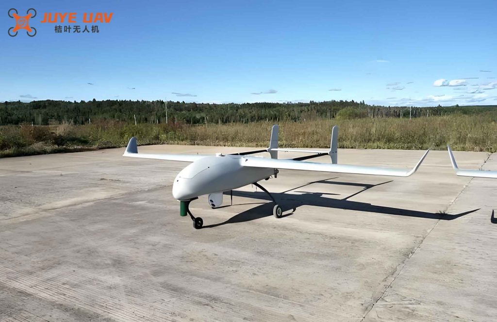
Fixed-wing UAVs have become indispensable in modern aerospace applications due to their exceptional endurance, stable flight characteristics, and extensive operational range. These attributes make them particularly suitable for strategic reconnaissance, environmental monitoring, surveying and mapping, and various other mission-critical operations. However, the control design for fixed-wing UAVs presents significant theoretical and practical challenges that stem from two fundamental characteristics: underactuation and parametric uncertainty.
The underactuated nature of fixed-wing UAVs arises from the fact that these systems possess six degrees of freedom but are controlled by only four control inputs. This inherent disparity between the number of degrees of freedom and the number of control inputs imposes fundamental constraints on the achievable motion patterns and complicates the trajectory tracking problem. Moreover, the aerodynamic parameters of fixed-wing UAVs, such as drag coefficients, moment of inertia, and actuator gains, are often imprecisely known or may vary during flight operations due to changing environmental conditions, payload variations, or structural degradation. This parametric uncertainty degrades control performance and can potentially compromise flight safety.
Existing approaches to address the underactuation problem in fixed-wing UAVs can be broadly categorized into inner-outer loop architectures, hierarchical decomposition methods, and transverse function techniques. In the inner-outer loop paradigm, the inner loop regulates attitude and altitude through optimal control or sliding mode methods, while the outer loop generates reference signals for the inner loop based on position errors. Hierarchical decomposition approaches partition the system into fully-actuated and underactuated subsystems, designing separate control laws for each subsystem. Transverse function methods introduce auxiliary variables to simultaneously stabilize multiple error states, thereby circumventing the underactuation constraint. While these methods have demonstrated varying degrees of success, they often lack rigorous guarantees for simultaneous convergence of all tracking errors.
Adaptive control has emerged as a powerful tool for handling parametric uncertainty in fixed-wing UAV systems. Classical adaptive control methods, including Lyapunov-based and estimation-based approaches, have been extensively studied. Lyapunov-based methods ensure stability through carefully designed adaptation laws, but they typically do not guarantee accurate parameter identification. Estimation-based methods, on the other hand, exploit excitation information contained in the system input-output data to estimate unknown parameters and can achieve parameter convergence under persistent excitation conditions. However, the persistent excitation condition is difficult to verify a priori and may not hold during regular flight operations.
Recent advances in data-driven adaptive control have led to the development of concurrent learning, composite learning, and regulation-triggered batch identification techniques that relax the excitation requirements. Concurrent learning methods employ excitation detection algorithms to collect informative data at specific time instants, but they may suffer from excitation遗漏 issues due to sampling limitations. Composite learning and regulation-triggered batch identification approaches utilize continuous integration to accumulate excitation information, ensuring richness of the collected data while introducing potential unboundedness of the regression equation. The challenge of maintaining boundedness while preserving directional excitation richness remains an open problem.
In the specific context of fixed-wing UAV control, several adaptive control frameworks have been proposed. These include parameterized model fitting combined with adaptive laws for uncertainty compensation, composite learning-based attitude control with relaxed excitation conditions, and hierarchical backstepping sliding mode controllers with gradient-based adaptation. Despite these advances, existing methods often fail to simultaneously achieve satisfactory tracking performance, accurate parameter estimation, and rigorous stability guarantees under practical excitation conditions.
To address these limitations, we propose a novel composite control framework that integrates unicycle-based model transformation for underactuation handling, backstepping fixed-time hierarchical control for trajectory tracking, spectral decomposition-based linear regression equation construction for excitation information accumulation, and regulation-triggered batch identification for parameter estimation. The main contributions of this work are threefold:
First, compared with existing works that address the underactuation problem in fixed-wing UAVs, our approach utilizes a unicycle model transformation combined with backstepping fixed-time hierarchical control to achieve zero-convergence of tracking errors, thereby enhancing tracking performance. Second, in contrast to existing excitation collection schemes, we employ spectral decomposition techniques to construct linear regression equations and design forgetting factors based on the eigenvalues of the excitation matrix. This approach ensures boundedness of the regression equation while accounting for directional differences in excitation richness. Third, unlike existing adaptive control methods for fixed-wing UAVs, our regulation-triggered batch identification technique decouples the underactuation problem from parametric uncertainty, eliminating the influence of unknown parameters through a finite number of parameter updates under non-persistent partial excitation conditions.
2. System Modeling and Problem Formulation
In this section, we present the mathematical model of the fixed-wing UAV and formulate the control problem. The kinematic model of the fixed-wing UAV in the horizontal plane can be described by the following equations:
$$
\begin{aligned}
\dot{x} &= v\cos\phi,\\
\dot{y} &= v\sin\phi,\\
\dot{v} &= a,\\
\dot{\phi} &= \omega_y,
\end{aligned}
$$
where $\mathbf{p}=[x,y]^T$ represents the position coordinates of the UAV, $\phi$ denotes the yaw angle, $v$ is the linear velocity, $\omega_y$ is the yaw angular velocity, and $a$ is the linear acceleration.
The dynamic model of the fixed-wing UAV captures the force and moment balance, which can be expressed as:
$$
\begin{aligned}
m\dot{v} &= T – \frac{1}{2}\rho_a Sv^2 C_D,\\
I_z\dot{\omega}_y &= \frac{1}{2}\rho_a v^2 Sb C_n \delta_r,
\end{aligned}
$$
where $m$ is the mass of the UAV, $\rho_a$ is the air density, $S$ is the wing area, $C_D$ is the drag coefficient, $I_z$ is the moment of inertia about the $z$-axis, $b$ is the wingspan, $C_n$ is the rudder moment coefficient, $T$ is the engine thrust, and $\delta_r$ is the rudder deflection angle. The control inputs $T$ and $\delta_r$ are related to the commanded values $T_c$ and $\delta_{rc}$ through the linear relationships $T = k_1 T_c$ and $\delta_r = k_2 \delta_{rc}$, where $k_1$ and $k_2$ are the thrust coefficient and servo transmission coefficient, respectively.
In this work, we assume that the parameters $k_1$, $k_2$, $C_D$, $C_n$, and $I_z$ are unknown constant parameters. To facilitate adaptive control design, we perform a linear parameterization of the dynamic model, yielding:
$$
\dot{\mathbf{s}} = \mathbf{\Psi}(\mathbf{s},\mathbf{u})^T \boldsymbol{\theta},
$$
where $\mathbf{s}=[v,\omega_y]^T$ is the state vector, $\mathbf{\Psi}(\mathbf{s},\mathbf{u})$ is the nonlinear regression matrix, and $\boldsymbol{\theta}$ is the vector of unknown parameters, given by:
$$
\mathbf{\Psi}(\mathbf{s},\mathbf{u}) = \begin{pmatrix}
-\frac{\rho_a Sv^2}{2m} & 0 \\
0 & \frac{\rho_a v^2 Sb}{2I_z}
\end{pmatrix}, \quad
\boldsymbol{\theta} = \begin{pmatrix}
\theta_1 \\
\theta_2 \\
\theta_3
\end{pmatrix} = \begin{pmatrix}
C_D \\
k_1 \\
k_2 C_n / I_z
\end{pmatrix}.
$$
Due to the product form of the unknown parameters $k_2$, $C_n$, and $I_z$, they are treated as a single composite parameter denoted by $\theta_3$.
The fixed-wing UAV model described above presents two fundamental challenges for control design. First, the system is underactuated, as there are three outputs $(x, y, \phi)$ but only two control inputs $(T_c, \delta_{rc})$. Second, the dynamic model contains parametric uncertainty, which affects both the translational and rotational dynamics.
The control objectives of this work are threefold. First, the position coordinates of the fixed-wing UAV should accurately track a reference trajectory, with the tracking error converging to zero. Second, all spectra of the regression term $\mathbf{\Psi}$ should be collected into the linear regression equation $\mathbf{Z}(t) = \mathbf{W}(t)\boldsymbol{\theta}$, while maintaining the boundedness of the equation. Third, the influence of parametric uncertainty in the dynamic model should be eliminated after a finite number of parameter updates.
To facilitate the subsequent controller design and stability analysis, we introduce the following assumptions and lemmas.
Assumption 1. The reference trajectory $\mathbf{p}_r(t)$ is bounded and twice continuously differentiable. There exists a positive constant $M$ such that $|\mathbf{p}_r(t)| \leq M$ for all $t \geq 0$, and $\dot{\mathbf{p}}_r(t)$, $\ddot{\mathbf{p}}_r(t)$ exist and are continuous.
Assumption 2. There exists a known set $\mathcal{B} \subset \mathbb{R}$ such that $k_1, k_2 \in \mathcal{B}$ and $0 \notin \mathcal{B}$. This assumption prevents the control inputs from becoming singular during the adaptation process.
Lemma 1 (Fixed-Time Stability). For a positive definite function $V(\zeta)$, if there exist constants $\varepsilon_1 > 0$, $\varepsilon_2 > 0$, $0 < r_1 < 1$, and $r_2 > 1$ such that $\dot{V}(\zeta) = -\varepsilon_1 V^{r_1}(\zeta) – \varepsilon_2 V^{r_2}(\zeta)$, then $V(\zeta)$ converges to zero within a fixed time, and the convergence time is bounded by:
$$
T_{\max} = \frac{1}{\varepsilon_1(1-r_1)} + \frac{1}{\varepsilon_2(r_2-1)}.
$$
Lemma 2 (Spectral Decomposition). Consider an $n$-dimensional normal matrix $\mathbf{W}$ with $h$ distinct eigenvalues $\lambda_1, \lambda_2, \ldots, \lambda_h$. Let $\mathbf{e}_{i,1}, \mathbf{e}_{i,2}, \ldots, \mathbf{e}_{i,k_i}$ be a set of orthonormal basis vectors for the eigenspace associated with eigenvalue $\lambda_i$. Then the spectral projector $\mathbf{E}_i$ is defined as $\mathbf{E}_i = \sum_{j=1}^{k_i} \mathbf{e}_{i,j}\mathbf{e}_{i,j}^T$, and the spectral decomposition of $\mathbf{W}$ takes the form $\mathbf{W} = \sum_{i=1}^h \lambda_i \mathbf{E}_i$. The spectral projector set $\{\mathbf{E}_1, \mathbf{E}_2, \ldots, \mathbf{E}_h\}$ is unique and satisfies the properties: $\sum_{i=1}^h \mathbf{E}_i = \mathbf{I}$, $\mathbf{E}_i^2 = \mathbf{E}_i$ for all $i$, and $\mathbf{E}_i\mathbf{E}_j = \mathbf{0}$ for $i \neq j$.
3. Controller Design
The proposed controller design proceeds in four stages: model transformation for underactuation handling, adaptive backstepping fixed-time control design, linear regression equation construction via spectral decomposition, and regulation-triggered batch parameter estimation.
3.1 Model Transformation
To address the underactuation problem, we adopt a unicycle model transformation approach. From the kinematic equations, we have $\dot{x} = v\cos\phi$ and $\dot{y} = v\sin\phi$. Defining the velocity components $v_x = \dot{x}$ and $v_y = \dot{y}$, their time derivatives are:
$$
\begin{aligned}
\dot{v}_x &= \dot{v}\cos\phi – v\dot{\phi}\sin\phi,\\
\dot{v}_y &= \dot{v}\sin\phi + v\dot{\phi}\cos\phi.
\end{aligned}
$$
By introducing virtual control inputs $u_x = \dot{v}_x$ and $u_y = \dot{v}_y$, we can establish the following transformation relationship:
$$
\begin{pmatrix}
\omega_y \\
a
\end{pmatrix} = \begin{pmatrix}
-\frac{u_x\sin\phi + u_y\cos\phi}{v} \\
u_x\cos\phi + u_y\sin\phi
\end{pmatrix}.
$$
Let $\boldsymbol{\upsilon} = [v_x, v_y]^T$ denote the velocity vector and $\mathbf{u}_v = [u_x, u_y]^T$ denote the virtual control input vector. The transformed kinematic model becomes:
$$
\begin{aligned}
\dot{\mathbf{p}} &= \boldsymbol{\upsilon},\\
\dot{\boldsymbol{\upsilon}} &= \mathbf{u}_v.
\end{aligned}
$$
This transformation effectively converts the original underactuated system into a fully-actuated double-integrator system in the Cartesian coordinates. The underactuation problem is thereby resolved, as the two control inputs $u_x$ and $u_y$ can now directly regulate the two position outputs $x$ and $y$, provided that the yaw angle $\phi$ is measurable.
3.2 Adaptive Backstepping Fixed-Time Control Design
Based on the transformed model, we employ a backstepping approach combined with fixed-time control techniques to design the control law. The design procedure consists of two steps.
Step 1: Virtual Control Design. Define the tracking errors:
$$
\begin{aligned}
\mathbf{z}_1 &= \mathbf{p} – \mathbf{p}_r,\\
\mathbf{z}_2 &= \boldsymbol{\upsilon} – \boldsymbol{\alpha},
\end{aligned}
$$
where $\boldsymbol{\alpha}$ is a stabilizing function to be designed. The derivative of $\mathbf{z}_1$ is $\dot{\mathbf{z}}_1 = \boldsymbol{\upsilon} – \dot{\mathbf{p}}_r$. Consider the Lyapunov function candidate $V_1 = \frac{1}{2}\mathbf{z}_1^T\mathbf{z}_1$. Its time derivative is $\dot{V}_1 = \mathbf{z}_1^T(\mathbf{z}_2 + \boldsymbol{\alpha} – \dot{\mathbf{p}}_r)$. To stabilize $\mathbf{z}_1$, we design the stabilizing function as:
$$
\boldsymbol{\alpha} = -c_1\mathbf{z}_1 + \dot{\mathbf{p}}_r,
$$
where $c_1 > 0$ is a design parameter. Substituting this expression yields $\dot{V}_1 = -c_1\mathbf{z}_1^T\mathbf{z}_1 + \mathbf{z}_1^T\mathbf{z}_2$.
Step 2: Virtual Control Implementation. The derivative of $\mathbf{z}_2$ is $\dot{\mathbf{z}}_2 = \mathbf{u}_v + c_1(\boldsymbol{\upsilon} – \dot{\mathbf{p}}_r) – \ddot{\mathbf{p}}_r$. Consider the augmented Lyapunov function $V_2 = V_1 + \frac{1}{2}\mathbf{z}_2^T\mathbf{z}_2$. Its time derivative is:
$$
\dot{V}_2 = -c_1\mathbf{z}_1^T\mathbf{z}_1 + \mathbf{z}_2^T(\mathbf{z}_1 + \mathbf{u}_v + c_1\boldsymbol{\upsilon} – c_1\dot{\mathbf{p}}_r – \ddot{\mathbf{p}}_r).
$$
We design the desired virtual control input $\mathbf{u}_{vr}$ as:
$$
\mathbf{u}_{vr} = -c_2\mathbf{z}_2 – \mathbf{z}_1 – c_1\boldsymbol{\upsilon} + c_1\dot{\mathbf{p}}_r + \ddot{\mathbf{p}}_r,
$$
where $c_2 > 0$ is a design parameter. When $\mathbf{u}_v$ converges to $\mathbf{u}_{vr}$, the Lyapunov function derivative becomes $\dot{V}_2 = -c_1\mathbf{z}_1^T\mathbf{z}_1 – c_2\mathbf{z}_2^T\mathbf{z}_2$, which guarantees exponential convergence of the tracking errors.
From the desired virtual control $\mathbf{u}_{vr} = [u_{xr}, u_{yr}]^T$, we can compute the desired yaw angular velocity $\omega_{yr}$ and linear acceleration $a_r$ using the transformation:
$$
\begin{pmatrix}
\omega_{yr} \\
a_r
\end{pmatrix} = \begin{pmatrix}
-\frac{u_{xr}\sin\phi + u_{yr}\cos\phi}{v} \\
u_{xr}\cos\phi + u_{yr}\sin\phi
\end{pmatrix}.
$$
Since the velocity $v$ of the fixed-wing UAV is always positive during flight, the angular velocity computation does not exhibit singularity.
Step 3: Fixed-Time Control Design. Define the angular velocity tracking error $z_3 = \omega_y – \omega_{yr}$ and consider the Lyapunov function $V_3 = \frac{1}{2}z_3^2$. Its derivative is $\dot{V}_3 = z_3(\alpha_y – \dot{\omega}_{yr})$, where $\alpha_y$ is the yaw angular acceleration. Based on Lemma 1, we design the desired yaw angular acceleration $\alpha_{yr}$ as:
$$
\alpha_{yr} = -c_3|z_3|^{\beta_1}\text{sgn}(z_3) – c_4|z_3|^{\beta_2}\text{sgn}(z_3) + \dot{\omega}_{yr},
$$
where $c_3 > 0$, $c_4 > 0$, $0 < \beta_1 < 1$, and $\beta_2 > 1$ are design parameters. This control law ensures that $V_3$ satisfies $\dot{V}_3 = -c_3|z_3|^{\beta_1+1} – c_4|z_3|^{\beta_2+1}$, which implies fixed-time convergence of $z_3$ to zero.
The actual control inputs $T_c$ and $\delta_{rc}$ are obtained by combining the dynamic model inversion with the parameter estimates:
$$
\begin{pmatrix}
T_c \\
\delta_{rc}
\end{pmatrix} = \begin{pmatrix}
\frac{m a_r + \frac{1}{2}\rho_a S v^2 \hat{\theta}_1}{\hat{\theta}_2} \\
\frac{2I_z \alpha_{yr}}{\rho_a v^2 S b \hat{\theta}_3}
\end{pmatrix},
$$
where $\hat{\boldsymbol{\theta}} = [\hat{\theta}_1, \hat{\theta}_2, \hat{\theta}_3]^T$ are the parameter estimates provided by the regulation-triggered batch identifier.
3.3 Linear Regression Equation Construction
To enable parameter estimation, we construct a linear regression equation $\mathbf{Z}(t) = \mathbf{W}(t)\boldsymbol{\theta}$ using spectral decomposition techniques. The excitation matrix $\mathbf{W}(t)$ collects spectral information from the regression term $\mathbf{\Psi}(\mathbf{s},\mathbf{u})$. Applying Lemma 2, the spectral decomposition of $\mathbf{W}$ can be expressed as $\mathbf{W}(t) = \sum_{i=1}^{h(t)} \lambda_i(t)\mathbf{E}_i(t)$.
Using the orthogonality property of the spectral projectors $\mathbf{E}_i$, the linear regression equation can be decomposed into $h(t)$ different excitation directions:
$$
\mathbf{E}_i(t)\mathbf{Z}(t) = \lambda_i(t)\mathbf{E}_i(t)\boldsymbol{\theta}, \quad i = 1, 2, \ldots, h(t).
$$
Multiplying both sides of the dynamic equation by $\mathbf{\Psi}(\mathbf{s},\mathbf{u})$ and combining with the decomposed regression equation, we construct the following forgetting law:
$$
\begin{aligned}
\dot{\mathbf{Z}} &= \mathbf{\Psi}(\mathbf{s},\mathbf{u})\mathbf{s} – \sum_{i=1}^{h(t)} \rho_i(\lambda_i)\mathbf{E}_i(t)\mathbf{Z},\\
\dot{\mathbf{W}} &= \mathbf{\Psi}(\mathbf{s},\mathbf{u})\mathbf{\Psi}^T(\mathbf{s},\mathbf{u}) – \sum_{i=1}^{h(t)} \rho_i(\lambda_i)\lambda_i(t)\mathbf{E}_i(t),
\end{aligned}
$$
with initial conditions $\mathbf{Z}(0) = \mathbf{0}$ and $\mathbf{W}(0) = \mathbf{0}$. The forgetting factor $\rho_i(\lambda_i)$ is designed based on the eigenvalues of the excitation matrix:
$$
\rho_i(\lambda_i) = \begin{cases}
0, & \text{if } \lambda_i \leq \sigma_{\min},\\
\text{sat}\left(\frac{\lambda_i}{\lambda_{\max}(\mathbf{\Psi}\mathbf{\Psi}^T)} – \mu\right) \eta, & \text{otherwise},
\end{cases}
$$
where $\lambda_{\max}(\mathbf{\Psi}\mathbf{\Psi}^T)$ is the maximum eigenvalue of $\mathbf{\Psi}\mathbf{\Psi}^T$, $\sigma_{\min}$ and $\sigma_{\max}$ are the thresholds for the forgetting activation, $\mu = (\sigma_{\max} + \sigma_{\min})/2$ is the center of the saturation function, and $\eta = (\sigma_{\max} – \sigma_{\min})/2$ is the width. The saturation function $\text{sat}(\cdot)$ is defined as:
$$
\text{sat}(x) = \begin{cases}
-1, & x \leq -1,\\
x, & -1 < x < 1,\\
1, & x \geq 1.
\end{cases}
$$
The forgetting factor $\rho_i(\lambda_i)$ ensures that excitation information in directions with $\lambda_i \leq \sigma_{\min}$ is preserved, while information in directions with $\lambda_i > \sigma_{\min}$ is forgotten at a rate proportional to $\rho_i(\lambda_i)$. This mechanism maintains the boundedness of the regression equation while preserving the richness of the collected excitation information.
The properties of the constructed linear regression equation are summarized in the following theorem.
Theorem 1. Consider the dynamic model with parametric uncertainty and the constructed linear regression equation. The following conclusions hold:
1) The excitation matrix $\mathbf{W}(t)$ is positive semidefinite for all $t \geq 0$.
2) If the regression term $\mathbf{\Psi}(\mathbf{s},\mathbf{u})$ is bounded, then the eigenvalues of $\mathbf{W}$ are bounded, with the upper bound being $\sigma_{\max}$.
3) For any time instant $\tau \in [0, t]$, the column space of $\mathbf{\Psi}(\mathbf{s}(\tau),\mathbf{u}(\tau))$ is a subset of the column space of $\mathbf{W}(t)$.
4) For a constant vector $\boldsymbol{\varphi}$, the condition $\mathbf{W}(t)\boldsymbol{\varphi} = \mathbf{0}$ is equivalent to $\mathbf{\Psi}^T(\mathbf{s}(\tau),\mathbf{u}(\tau))\boldsymbol{\varphi} = \mathbf{0}$ for all $\tau \in [0, t]$.
Theorem 1 establishes that all past excitation information is accumulated in the matrix $\mathbf{W}$, and the null space $\mathcal{N}(\mathbf{W}(t))$ represents the unexcited subspace of the parameter estimation error, while the range space $\mathcal{R}(\mathbf{W}(t))$ represents the excited subspace. An increase in the rank of $\mathbf{W}(t)$ indicates that new excitation information has been collected, reducing the dimensionality of the unexcited subspace.
3.4 Regulation-Triggered Batch Identifier
Based on the constructed linear regression equation, we design a regulation-triggered batch identifier that updates the parameter estimates at discrete time instants when certain trigger conditions are met. The parameter update law is given by:
$$
\hat{\boldsymbol{\theta}}(\tau_i) = \arg\min_{\boldsymbol{\Theta} \in \mathcal{B} \times \mathbb{R}} \|\boldsymbol{\Theta} – \hat{\boldsymbol{\theta}}(\tau_{i-1})\|^2, \quad \text{s.t. } \mathbf{Z}(\tau_i) = \mathbf{W}(\tau_i)\boldsymbol{\Theta},
$$
where $\tau_i$ denotes the $i$-th trigger instant. The parameter estimate $\hat{\boldsymbol{\theta}}$ is updated at time $\tau_i$ using the excitation information collected over the interval $[0, \tau_i]$, and remains constant between consecutive trigger instants:
$$
\hat{\boldsymbol{\theta}}(t) = \hat{\boldsymbol{\theta}}(\tau_i), \quad \forall t \in [\tau_i, \tau_{i+1}).
$$
The constraint $\boldsymbol{\Theta} \in \mathcal{B} \times \mathbb{R}$ ensures that the estimated parameters $\hat{\theta}_2$ and $\hat{\theta}_3$ never approach zero, thereby preventing control input singularity. The parameter estimate $\hat{\boldsymbol{\theta}}(\tau_i)$ is the closest point to the previous estimate $\hat{\boldsymbol{\theta}}(\tau_{i-1})$ within the intersection of the set $\mathcal{B}$ and the hyperplane defined by the linear regression equation.
To determine the trigger instants, we design a regulation-triggered condition that activates the parameter update when either the control performance degrades beyond a threshold, a maximum time interval has elapsed, or the collected excitation information becomes significantly richer than at the previous update. The trigger condition is:
$$
\tau_i = \begin{cases}
t, & \text{if } V_3(t) = \chi_i, \text{ or } t = \tau_{i-1} + T, \text{ or } K_{\mathbf{W}}^l(\tau_i) > K_{\mathbf{W}}^l(\tau_{i-1}),
\end{cases}
$$
where $T > 0$ is the maximum trigger interval, $V_3$ is the Lyapunov function for the fixed-time control, $K_{\mathbf{W}}^l(t)$ denotes the number of eigenvalues of the excitation matrix $\mathbf{W}$ that are greater than a threshold $l$, and $\chi_i$ is the trigger threshold designed as:
$$
\chi_i = \gamma_1 V_3(\tau_{i-1}) + \gamma_2, \quad \gamma_1 \geq 1, \gamma_2 > 0,
$$
with $\chi_i > V_3(\tau_{i-1})$ to ensure strict improvement. The initial trigger instant is set as $\tau_0 = 0$ s.
The regulation-triggered batch identifier ensures that parameter updates occur only when necessary, either due to performance degradation, time-triggered supervision, or detection of new excitation information. This approach minimizes unnecessary computational burden while guaranteeing parameter convergence.
4. Stability Analysis
In this section, we present the main theoretical results of this work, which characterize the stability, convergence, and parameter identification properties of the closed-loop system.
Theorem 2. Consider the fixed-wing UAV system described by the dynamic model with parametric uncertainty, controlled by the proposed adaptive hierarchical control law with the regulation-triggered batch identifier. Under Assumptions 1 and 2, the following conclusions hold:
1) The number of parameter estimate updates does not exceed 3.
2) Let $\tau_k$ be the final update instant of the parameter estimate. Then, for all $t \geq \tau_k$, the influence of the unknown parameters is completely eliminated, i.e., $\mathbf{\Psi}^T(\mathbf{s}(t),\mathbf{u}(t))\tilde{\boldsymbol{\theta}} \equiv 0$, where $\tilde{\boldsymbol{\theta}} = \hat{\boldsymbol{\theta}} – \boldsymbol{\theta}$.
3) The closed-loop system is stable, and the tracking errors converge to zero.
4) The system does not exhibit Zeno behavior, i.e., no infinite number of parameter updates occur in finite time.
Proof 1. Let $\mathcal{R}(\mathbf{W}(\tau_i))$ and $\mathcal{N}(\mathbf{W}(\tau_i))$ denote the range space and null space of $\mathbf{W}$ at time $\tau_i$, respectively. When the trigger condition is activated and $\hat{\boldsymbol{\theta}}(\tau_{i-1}) \notin \mathcal{N}(\mathbf{W}(\tau_i))$, the parameter estimate must be updated to ensure $\hat{\boldsymbol{\theta}}(\tau_i) \in \mathcal{N}(\mathbf{W}(\tau_i))$. Since new excitation information is collected between consecutive trigger instants, the rank of $\mathbf{W}$ increases, i.e., $\dim(\mathcal{R}(\mathbf{W}(\tau_i))) \geq \dim(\mathcal{R}(\mathbf{W}(\tau_{i-1}))) + 1$, and consequently $\dim(\mathcal{N}(\mathbf{W}(\tau_i))) \leq \dim(\mathcal{N}(\mathbf{W}(\tau_{i-1}))) – 1$. By the monotone convergence theorem, $\dim(\mathcal{N}(\mathbf{W}(\tau_i)))$ eventually decreases to a non-negative integer. Since $\dim(\mathcal{N}(\mathbf{W}(0))) = 3$, the number of parameter estimate updates does not exceed 3.
Proof 2. If there exists a time instant $t \geq \tau_k$ such that $\mathbf{\Psi}^T(\mathbf{s}(t),\mathbf{u}(t))\tilde{\boldsymbol{\theta}} \neq \mathbf{0}$, then new excitation information would be available, requiring further parameter updates according to the trigger condition. This contradicts the definition of $\tau_k$ as the final update instant. Therefore, $\mathbf{\Psi}^T(\mathbf{s}(t),\mathbf{u}(t))\tilde{\boldsymbol{\theta}} \equiv \mathbf{0}$ for all $t \geq \tau_k$, meaning the influence of the unknown parameters is completely eliminated.
Proof 3. With the control law incorporating accurate parameter estimates after $\tau_k$, the fixed-time control design ensures that $V_3$ converges to zero within a fixed time, i.e., $z_3$ converges to zero. Consequently, the actual virtual control inputs $(u_x, u_y)$ converge to their desired values $(u_{xr}, u_{yr})$, and the backstepping design guarantees exponential convergence of the tracking errors $\mathbf{z}_1$ and $\mathbf{z}_2$ to zero. Thus, the closed-loop system is stable and the tracking errors converge to zero.
Proof 4. The trigger condition consists of three types: (i) performance-triggered when $V_3(t) = \chi_i$, (ii) periodic-triggered when $t = \tau_{i-1} + T$, and (iii) excitation-richness-triggered when $K_{\mathbf{W}}^l(\tau_i) > K_{\mathbf{W}}^l(\tau_{i-1})$. For types (i) and (iii), parameter updates are accompanied by an increase in the rank of $\mathbf{W}$, which, as proven in part 1, can occur at most 3 times. For type (ii), the minimum time interval between triggers is $T > 0$. Therefore, none of the three trigger types can cause an infinite number of parameter updates in finite time, precluding Zeno behavior.
The theoretical analysis demonstrates that the proposed control framework achieves simultaneous tracking error convergence, parameter identification, and closed-loop stability without requiring persistent excitation conditions. The key advantage of the regulation-triggered batch identification approach is that it decouples the underactuation problem from the parametric uncertainty problem, allowing each to be addressed with specialized techniques.
5. Simulation Results
To validate the effectiveness of the proposed control framework, we conduct numerical simulations of the fixed-wing UAV tracking control problem. The simulation parameters are selected as follows.
Table 1: Controller Design Parameters
| Parameter | Symbol | Value |
|---|---|---|
| Backstepping gain 1 | $c_1$ | 0.8 |
| Backstepping gain 2 | $c_2$ | 0.8 |
| Fixed-time control gain 1 | $c_3$ | 1.0 |
| Fixed-time control gain 2 | $c_4$ | 1.0 |
| Fixed-time exponent 1 | $\beta_1$ | 0.6 |
| Fixed-time exponent 2 | $\beta_2$ | 1.2 |
| Trigger scaling factor 1 | $\gamma_1$ | 5.0 |
| Trigger scaling factor 2 | $\gamma_2$ | 1.5 |
| Forgetting lower bound | $\sigma_{\min}$ | 3.0 |
| Forgetting upper bound | $\sigma_{\max}$ | 8.0 |
| Minimum trigger interval | $T$ | 3 s |
Table 2: Fixed-Wing UAV Physical Parameters
| Parameter | Symbol | Value |
|---|---|---|
| Mass | $m$ | 0.55 kg |
| Air density | $\rho_a$ | 1.225 kg/m³ |
| Wing area | $S$ | 0.21 m² |
| Wingspan | $b$ | 1.37 m |
Table 3: True and Initial Estimated Parameters
| Parameter | True Value | Initial Estimate |
|---|---|---|
| $\theta_1$ | 0.015 | 0.03 |
| $\theta_2$ | 4.0 | 3.0 |
| $\theta_3$ | 0.3 | 0.5 |
The reference trajectory is specified as:
$$
\begin{aligned}
x_r(t) &= 5 – 10\cos(0.7t),\\
y_r(t) &= -10\sin(0.7t),
\end{aligned}
$$
which describes a circular path with radius 10 m centered at (5, 0).
The simulation results demonstrate the effectiveness of the proposed control framework. The actual trajectory of the fixed-wing UAV converges to the desired trajectory, with the initial deviation being gradually eliminated as the UAV moves along the reference path. The tracking errors in both the $x$ and $y$ directions exhibit a clear converging trend, indicating successful trajectory tracking.
Table 4: Comparison of Excitation Collection Methods
| Method | Excitation Richness | Boundedness of Regression Equation |
|---|---|---|
| Integrator-based | Rich | Not guaranteed |
| Integrator + General Forgetting | Poor | Guaranteed |
| Integrator + Directional Forgetting | Poor | Guaranteed |
| Spectral Decomposition + Directional Forgetting (Ours) | Rich | Guaranteed |
Table 5: Comparison of Adaptive Control Methods
| Method | Required Excitation Condition | Parameter Update Continuity |
|---|---|---|
| Concurrent Learning | Weak persistent excitation | Continuous |
| Composite Learning | Weak/Full/Non-persistent partial excitation | Continuous |
| Regulation-Triggered Batch (Ours) | Non-persistent partial excitation | Discrete |
The parameter estimates converge to their true values after three updates, as predicted by the theoretical analysis. The first parameter update occurs shortly after the initial time when the performance trigger threshold is reached. The second update occurs when new excitation information is detected through the excitation richness trigger. The third update finalizes the parameter identification process, after which all parameter estimates remain at their true values.
The velocity profile of the fixed-wing UAV stabilizes at approximately 7 m/s, which is consistent with the trajectory requirements. The control inputs, namely the throttle command $T_c$ and the rudder deflection command $\delta_{rc}$, remain within reasonable bounds after saturation limiting, with $T_c \in [0, 1]$ and $\delta_{rc} \in [-1, 1]$. Importantly, the saturation limits do not compromise system stability or tracking accuracy.
The simulation results confirm that the proposed control algorithm successfully accomplishes the trajectory tracking task while eliminating the influence of parametric uncertainty. The finite-time convergence of the tracking errors, the accurate identification of the unknown parameters, and the absence of Zeno behavior all validate the theoretical predictions.
6. Conclusion
In this work, we have presented a comprehensive adaptive hierarchical control framework for fixed-wing UAVs that systematically addresses the coupled challenges of underactuated dynamics and parametric uncertainty. The key contributions of this work are threefold.
First, we developed a unicycle-based model transformation that converts the original underactuated fixed-wing UAV model into a virtual integrator system, enabling the application of standard control design techniques. Combining this transformation with backstepping and fixed-time control, we established a hierarchical control architecture that guarantees trajectory tracking error convergence to zero. This approach provides superior tracking performance compared to existing methods that only ensure boundedness or asymptotic convergence.
Second, we introduced a spectral decomposition-based linear regression equation construction method that quantitatively collects excitation information while maintaining boundedness of the regression equation. By designing forgetting factors based on the eigenvalues of the excitation matrix, our approach accounts for directional differences in excitation richness, ensuring that weakly excited directions are preserved while strongly excited directions are appropriately forgotten. This represents a significant improvement over existing integrator-based methods that either sacrifice excitation richness or fail to guarantee boundedness.
Third, we developed a regulation-triggered batch identifier that eliminates the influence of parametric uncertainty through a finite number of parameter updates under non-persistent partial excitation conditions. The discrete-time update mechanism, triggered by performance degradation, time-out, or detection of new excitation information, ensures computational efficiency while guaranteeing parameter convergence. The decoupling of the underactuation problem from the parametric uncertainty problem is a distinctive feature of our approach.
Future research directions include extending the proposed framework to handle external disturbances, which are prevalent in real-world flight operations. Additionally, we aim to adapt the control architecture to multi-agent systems, where multiple fixed-wing UAVs must coordinate their motions while dealing with individual parametric uncertainties. The extension to three-dimensional flight scenarios, incorporating altitude control and more complex aerodynamic effects, represents another promising avenue for future investigation.
In summary, the proposed adaptive hierarchical control framework provides a systematic solution to the trajectory tracking problem for fixed-wing UAVs with underactuated dynamics and parametric uncertainty. By unifying error convergence, excitation richness, and parameter identification accuracy within a single coherent framework, our approach advances the state of the art in fixed-wing UAV control and offers practical benefits for a wide range of aerospace applications.