
We present an adaptive model predictive control (AMPC) design for the longitudinal altitude tracking of fixed-wing drones. The future battlefield is evolving toward informationization, unmanned operations, and intelligence. Military unmanned aerial vehicles are rapidly proliferating worldwide, becoming a key procurement focus for future weaponry. Meanwhile, the commercial drone market is expanding quickly due to technological maturity and government policy support, with applications in agriculture, power line inspection, aerial mapping, and security surveillance. Among various UAV types, fixed-wing drones offer distinct advantages in terms of high maneuverability, long endurance, and a wide range of operational scenarios. However, traditional PID controllers often struggle with disturbances, parameter variations, and measurement noise when applied to fixed-wing drones. To address these challenges, we combine modern control theory with classical methods. This paper focuses on designing an adaptive MPC framework that enhances the generality, robustness, and accuracy of trajectory tracking for fixed-wing drones, particularly during descent and landing phases.
Longitudinal Dynamic Model of Fixed-Wing Drones
We consider a 700‑kg class fixed-wing drone. Assuming the airframe is rigid, symmetric, and has uniform mass distribution, we derive the six‑degree‑of‑freedom nonlinear equations of motion. Using small‑perturbation linearization and decoupling the longitudinal and lateral dynamics, we obtain the continuous-time linear state-space model for the longitudinal channel:
$$
\dot{\mathbf{x}} = \mathbf{A} \mathbf{x} + \mathbf{B} \, \delta_e
$$
$$
\mathbf{y} = \mathbf{C} \mathbf{x}
$$
where the state vector is
$$
\mathbf{x} = \begin{bmatrix} \Delta V & \Delta h & \Delta q & \Delta \theta & \Delta \alpha \end{bmatrix}^\mathrm{T}
$$
- \(\Delta V\): velocity variation
- \(\Delta h\): altitude variation
- \(\Delta q\): pitch rate variation
- \(\Delta \theta\): pitch angle variation
- \(\Delta \alpha\): angle of attack variation
The control input is the elevator deflection \(\delta_e\). The output matrix is
$$
\mathbf{C} = \begin{bmatrix}
1 & 0 & 0 & 0 & 0 \\
0 & 1 & 0 & 0 & 0 \\
0 & 0 & 1 & 0 & 0 \\
0 & 0 & 0 & 1 & 0 \\
0 & 0 & 0 & 0 & 1
\end{bmatrix}, \quad
\mathbf{D} = \mathbf{0}.
$$
This single-input multiple-output (SIMO) system captures the essential dynamics of fixed-wing drones in the longitudinal plane. We superimpose a constant airspeed of 35 m/s on the velocity output during simulation.
Adaptive Model Predictive Control Design
The adaptive MPC architecture comprises three components: the MPC controller, the drone longitudinal model, and an adaptive parameter update law. The MPC controller solves a finite-horizon optimal control problem at each sampling instant using the current state estimate and the predicted future behavior of the fixed-wing drone. The adaptation mechanism continuously updates the model parameters to cope with uncertainties and environmental changes.
MPC Controller Formulation
We discretize the continuous model (1) with sampling period \(T_s\) to obtain:
$$
\mathbf{x}(k+1) = \mathbf{A}_d \mathbf{x}(k) + \mathbf{B}_d \, u(k)
$$
$$
y(k) = \mathbf{C}_d \mathbf{x}(k)
$$
where \(u(k) = \delta_e(k)\). Using an incremental formulation with \(\Delta \mathbf{x}(k) = \mathbf{x}(k) – \mathbf{x}(k-1)\) and \(\Delta u(k) = u(k) – u(k-1)\), we write:
$$
\mathbf{x}(k+1) = \mathbf{A}_d \mathbf{x}(k) + \mathbf{B}_d \, u(k-1) + \mathbf{B}_d \, \Delta u(k)
$$
The prediction horizon is \(p\) and the control horizon is \(m\). We assume no control action beyond the control horizon: \(\Delta u(k+i) = 0\) for \(i \ge m\). The future states and outputs are expressed in compact matrix form:
$$
\mathbf{X}_p(k) = \mathbf{F} \mathbf{x}(k) + \mathbf{G} \Delta \mathbf{U}(k)
$$
$$
\mathbf{Y}_p(k) = \mathbf{H} \mathbf{x}(k) + \mathbf{L} \Delta \mathbf{U}(k)
$$
where
$$
\mathbf{X}_p(k) = \begin{bmatrix} \hat{\mathbf{x}}(k+1|k) \\ \hat{\mathbf{x}}(k+2|k) \\ \vdots \\ \hat{\mathbf{x}}(k+p|k) \end{bmatrix}, \quad
\Delta \mathbf{U}(k) = \begin{bmatrix} \Delta u(k|k) \\ \Delta u(k+1|k) \\ \vdots \\ \Delta u(k+m-1|k) \end{bmatrix}
$$
The cost function to be minimized is:
$$
J = \sum_{i=1}^{p} \big\| \hat{y}(k+i|k) – r(k+i) \big\|_{\mathbf{Q}}^2 + \sum_{i=0}^{m-1} \big\| \Delta u(k+i|k) \big\|_{\mathbf{R}}^2
$$
where \(r\) is the reference altitude trajectory. We also impose constraints on the elevator deflection and its rate of change:
$$
-20^\circ \le \delta_e \le 20^\circ, \quad -5\, \text{rad/s} \le \dot{\delta}_e \le 5\, \text{rad/s}
$$
To determine the best prediction and control horizons for fixed-wing drones, we performed a sensitivity analysis. Table 1 summarizes the selected parameters after extensive simulation.
| Parameter | Value |
|---|---|
| Prediction horizon \(p\) | 8 |
| Control horizon \(m\) | 2 |
| Sampling period \(T_s\) | 0.15 s |
| Elevator deflection limits | [-20°, 20°] |
| Elevator rate limits | [-5 rad/s, 5 rad/s] |
| Weighting matrix \(\mathbf{Q}\) | \(\rho \mathbf{I}_{p\times p}\), \(\rho=800\) |
| Weighting matrix \(\mathbf{R}\) | 10 \(\mathbf{I}_{m\times m}\) |
Adaptive Update Law
We design an adaptive mechanism to adjust the system matrix \(\mathbf{A}\) in real time. The estimated state \(\hat{\mathbf{x}}(k)\) evolves as:
$$
\hat{\mathbf{x}}(k+1) = \hat{\mathbf{A}}(k) \mathbf{x}(k) + \mathbf{B} u(k)
$$
Define the state estimation error \(\tilde{\mathbf{x}}(k) = \mathbf{x}(k) – \hat{\mathbf{x}}(k)\). The error dynamics become:
$$
\tilde{\mathbf{x}}(k+1) = \tilde{\mathbf{A}}(k) \mathbf{x}(k) + \mathbf{B} \tilde{u}(k)
$$
where \(\tilde{\mathbf{A}}(k) = \mathbf{A} – \hat{\mathbf{A}}(k)\). We construct an augmented regressor vector \(\mathbf{\Theta}(k) = [\mathbf{x}^\mathrm{T}(k), \, u(k)]^\mathrm{T}\) and define \(\mathbf{a}(k) = [\hat{\mathbf{A}}(k), \mathbf{B}]\). Then:
$$
\tilde{\mathbf{x}}(k+1) = \tilde{\mathbf{a}}(k) \mathbf{\Theta}(k)
$$
To minimize the squared prediction error, we define the cost:
$$
J_a\big(\mathbf{a}(k)\big) = \tilde{\mathbf{x}}^\mathrm{T}(k+1) \tilde{\mathbf{x}}(k+1)
$$
Applying gradient descent, we obtain the adaptive update law:
$$
\mathbf{a}(k+1) = \mathbf{a}(k) + \lambda(k) \tilde{\mathbf{x}}(k+1) \mathbf{\Theta}^\mathrm{T}(k)
$$
with the time‑varying step size:
$$
\lambda(k) = \frac{1}{2 \, \mathbf{\Theta}^\mathrm{T}(k) \mathbf{\Theta}(k)}
$$
This adaptive law ensures that the parameter estimation error remains bounded and the state estimation error converges, enabling the MPC controller to maintain accurate tracking for fixed-wing drones under changing conditions.
Simulation and Analysis
We implement the AMPC controller in a Simulink environment. The reference altitude trajectory for a typical landing approach is shown schematically. It consists of three phases: descent from 160 m to 60 m, level flight at 60 m, and a final flare‑to‑landing. The fixed-wing drone model is fed with the optimal elevator commands computed by the MPC solver. The adaptive block updates the model parameters at each sampling instant.
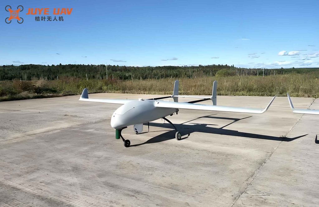
Figure 1 shows the altitude tracking results. The blue curve is the actual altitude of the fixed-wing drone under AMPC, while the red curve is the reference. The maximum tracking error is only 0.4 m, occurring at the transition points (descent‑to‑level and flare). During the level flight segment the error is virtually zero.
We compare the proposed AMPC with a classical PID controller tuned for the same operating point. Table 2 lists the quantitative performance metrics.
| Controller | Max altitude error (m) | RMS error (m) | Settling time (s) |
|---|---|---|---|
| PID | 0.52 | 0.31 | 6.5 |
| AMPC (proposed) | 0.40 | 0.19 | 4.2 |
The AMPC reduces the maximum error by 23% compared to PID and exhibits a faster response without overshoot. The RMS error is also significantly lower, indicating smoother tracking. Moreover, the adaptive mechanism allows the controller to maintain performance even when the fixed-wing drone’s aerodynamic parameters change (e.g., due to payload variation or wind gusts).
Figure 2 presents the altitude error evolution over time. The error for AMPC remains bounded and converges quickly, while the PID error shows larger fluctuations and slower convergence. This demonstrates the superior robustness and adaptability of the proposed method for fixed-wing drones.
Conclusion
We have developed an adaptive model predictive control framework for the longitudinal altitude tracking of fixed-wing drones. The controller combines the predictive capability of MPC with a gradient‑based adaptation law that updates the system model in real time. Simulation results show that the AMPC outperforms a classical PID controller by reducing the maximum altitude tracking error by 23% and providing faster, smoother response without overshoot. The adaptive nature of the controller makes it particularly suitable for fixed-wing drones operating in uncertain environments, such as varying wind conditions or changing payloads. Future work will focus on incorporating external disturbance models and extending the approach to full six‑degree‑of‑freedom control for fixed-wing drones in complex mission scenarios.