
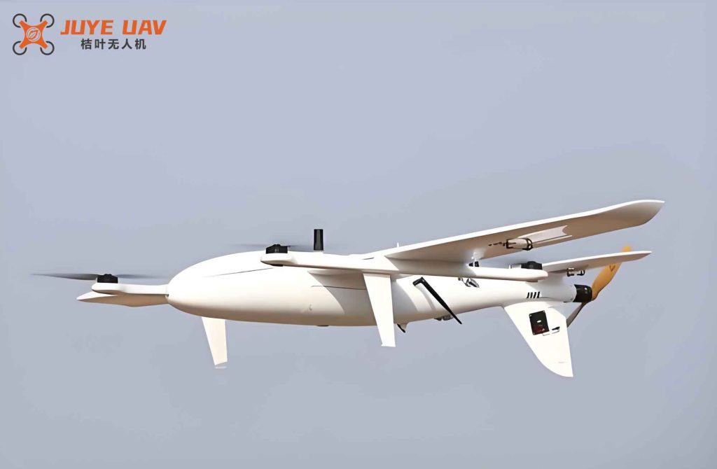
In our work, we focus on the challenging task of guiding fixed-wing drones to approach near-ground targets efficiently and safely, followed by a return to cruising altitude. Fixed-wing drones offer advantages such as high speed and long endurance, but their maneuverability is constrained by aerodynamic limitations. Traditional guidance algorithms, while effective for simple path following, often fail during transitions between multiple phases, leading to large maneuvers or energy inefficiency. Inspired by the hunting trajectories of raptors such as peregrine falcons and Harris’s hawks, we propose a composite optimal guidance framework that mimics the predator’s descent, capture, and recovery flight. This paper details our approach, which includes a bio-inspired trajectory optimization problem, a novel optimization solver combining Harris hawk foraging strategies with pigeon-inspired optimization, and a vector-field guidance law with collision avoidance. Comprehensive simulations demonstrate that our methods outperform conventional algorithms in both convergence speed and tracking accuracy for fixed-wing drone near-ground missions.
1. Problem Formulation: Bio-Inspired Trajectory Optimization
We model the raptor-inspired hunting trajectory as a two-phase motion: the descending phase toward a ground target and the ascending phase back to the initial altitude. The trajectory is parameterized by a set of scalar parameters \(k_h, a_h, c_h\) that define the shape. For the descending phase, the height profile is given by:
$$ z_h = -k_h x_h^2 (x_{h\infty} – (x_h – c_h))^2 \cdot \exp\left(-a_h \left( \text{Sat}((x_h – c_h) – x_t, z_{h0}) \right)^2 \right) $$
where \(\text{Sat}(\cdot)\) is a saturation function, \(x_t\) is the target position, \(z_{h0}\) is the initial height, and \(x_{h\infty}\) is the recovery point. The optimization goal is to minimize a cost function that balances mechanical energy change and flight time over both phases:
$$ J_d(k_h, a_h, c_h) = w_{e1} \Delta E_{s1} + w_{e2} \Delta E_{s2} + w_{t1} T_{s1} + w_{t2} T_{s2} $$
Here, \(\Delta E_{s1}\) and \(\Delta E_{s2}\) are the changes in mechanical energy during the first and second phases, and \(T_{s1}, T_{s2}\) are the corresponding flight times. The energy change for the first phase is computed as:
$$ \Delta E_{s1} = \frac{1}{2} m_h (v_{x,h,s1}^2 + v_{z,h,s1}^2) + m_h g z_{h,s1} – E_{h0} $$
where \(E_{h0}\) is the initial energy. Similarly, \(\Delta E_{s2}\) is defined. The velocities are derived from the trajectory shape with a sinusoidal modulation for the horizontal speed: \(\dot{x}_h = v_{xh} = A_v \sin(k_v t) + c_v\), and the vertical speed is obtained from the derivative of \(z_h\).
The optimization is subject to continuity constraints at the interface between phases:
$$ \begin{aligned} x_{h,s1}(end) &= x_t \\ z_{h,s1}(end) &= 0 \\ x_{h,s2}(end) &= x_{h\infty} \\ z_{h,s2}(end) &= z_{h0} \\ x_{h,s1}(end) &= x_{h,s2}(1) \\ z_{h,s1}(end) &= z_{h,s2}(1) \\ v_{x,h,s1}(end) &= v_{x,h,s2}(1) \\ v_{z,h,s1}(end) &= v_{z,h,s2}(1) \end{aligned} $$
Additionally, physical constraints such as speed limits and altitude bounds are enforced:
$$ \begin{aligned} v_{\min} &\leq \|\mathbf{v}\| \leq v_{\max} \\ a_{\min} &\leq \|\dot{\mathbf{v}}\| \leq a_{\max} \\ 0 &< z < h_{\max} \end{aligned} $$
To handle these constraints, we introduce slack variables \(\gamma\) and a quadratic penalty \(\Xi\), resulting in the augmented cost:
$$ J_n = J_d + w_\gamma (\gamma_{s1} + \gamma_{s2} + \gamma_{c1} + \gamma_{c2}) + w_c \Xi $$
Table 1 summarizes the key parameters used in our trajectory model.
| Parameter | Symbol | Value/Range |
|---|---|---|
| Initial altitude | \(z_{h0}\) | 60 m |
| Target altitude | \(z_t\) | 0 m |
| Recovery altitude | \(z_{h\infty}\) | 60 m |
| Maximum speed | \(v_{\max}\) | 30 m/s |
| Minimum speed | \(v_{\min}\) | 5 m/s |
| Maximum acceleration | \(a_{\max}\) | 10 m/s² |
| Minimum acceleration | \(a_{\min}\) | -10 m/s² |
| Slack variable bounds | \(\gamma\) | [-0.1, 0.1] |
2. Optimization Algorithm: Harris Hawk Improved Pigeon-Inspired Optimization
To solve the non-convex optimization problem, we developed a hybrid algorithm that combines the two-stage structure of pigeon-inspired optimization (PIO) with the hunting strategies of Harris’s hawks. The standard PIO has a map/compass operator and a landmark operator. The map/compass operator updates positions using:
$$ \begin{aligned} V_i(t+1) &= V_i(t) e^{-R(t+1)} + \text{rand} \cdot (X_{\text{gbest}}(t) – X_i(t)) \\ X_i(t+1) &= X_i(t) + V_i(t+1) \end{aligned} $$
where \(R\) is the exponential factor. After a certain number of iterations, the algorithm switches to the landmark operator:
$$ \begin{aligned} X_{\text{center}}(t) &= \frac{\sum_{i=1}^{M(t)} X_i(t) \text{fitness}(X_i(t))}{M(t) \sum_{i=1}^{M(t)} \text{fitness}(X_i(t))} \\ X_i(t+1) &= X_i(t) + \text{rand} \cdot (X_{\text{center}}(t) – X_i(t)) \\ M(t) &= \text{ceil}\left( \frac{M(t-1)}{2} \right) \end{aligned} $$
We observed that the landmark phase converges slowly. Inspired by the energy-based switching of Harris’s hawks during hunting, we introduced a search energy variable \(E\):
$$ E = 2 E_0 \left(1 – \frac{t}{t_{\max}}\right) $$
where \(E_0 \in (-1,1)\) is a random initial energy. When \(E > 1\), we retain the original landmark operator but without reducing population size. When \(E < 1\), we replace the landmark update with two modes based on the random variable \(q \in (0,1)\):
Soft siege (0.5 < E < 1):
$$ X_i(t+1) = \begin{cases} (X_{\text{gbest}}(t) – X_i(t)) – E |r_1 (X_{\text{gbest}}(t) – X_i(t))|, & q > 0.5 \\ X_{\text{gbest}}(t) – E |r_2 (X_{\text{gbest}}(t) – X_i(t))| + \mathbf{R}_D^l \times \text{LEVY}(D), & q \leq 0.5 \end{cases} $$
Hard siege (E ≤ 0.5):
$$ X_i(t+1) = \begin{cases} X_{\text{gbest}}(t) – E |X_{\text{gbest}}(t) – X_i(t)|, & q > 0.5 \\ X_{\text{gbest}}(t) – E |X_{\text{gbest}}(t) – X_i(t)| + \mathbf{R}_D^l \times \text{LEVY}(D), & q \leq 0.5 \end{cases} $$
Here, \(\text{LEVY}(D)\) is the Lévy flight function:
$$ \text{LEVY}(x) = 0.01 \times \frac{u \times \delta}{|v|^{1/\beta}}, \quad \delta = \left( \frac{\Gamma(1+\beta) \sin(\pi \beta / 2)}{\Gamma((1+\beta)/2) \times \beta \times 2^{(\beta-1)/2}} \right)^{1/\beta} $$
with \(\beta = 1.5\). The algorithm flow is summarized in Table 2.
| Step | Operation |
|---|---|
| 1 | Initialize pigeon population with random positions (parameters \(k_h, a_h, c_h\)) |
| 2 | Map/Compass Phase: Update velocity and position using Eq. (10) for \(N_{\text{map}}\) iterations |
| 3 | Compute energy \(E\) using Eq. (12); determine phase |
| 4 | Landmark Phase (modified): If \(E > 1\): use standard landmark (no population reduction) If \(0.5 < E \leq 1\): soft siege update (Eq. 13) If \(E \leq 0.5\): hard siege update (Eq. 15) |
| 5 | Evaluate fitness \(J_n\) for each pigeon; update global best |
| 6 | Repeat steps 2–5 until maximum iteration \(t_{\max}\) reached |
| 7 | Output optimal parameters \(k_h^*, a_h^*, c_h^*\) and the resulting trajectory |
We benchmarked HH-PIO against three standard algorithms: particle swarm optimization (PSO), genetic algorithm (GA), and original PIO. Table 3 shows the average cost function and optimization results over 200 independent runs.
| Algorithm | Mean cost | Mean energy gain (×10³) | Mean time (s) | Optimal parameters \((k_h, a_h, c_h)\) |
|---|---|---|---|---|
| HH-PIO (ours) | 5.3695 × 10⁵ | -3.8198 | 5.74 | 4.890×10⁻⁷, 7.833×10⁻⁸, 0.3498 |
| GA | 5.3655 × 10⁵ | -3.4676 | 7.86 | 4.890×10⁻⁷, 1.009×10⁻⁸, 0.4130 |
| PSO | 5.3755 × 10⁵ | -3.4663 | 3.99 | 4.890×10⁻⁷, 1.205×10⁻⁶, 0.4916 |
| PIO | 5.5391 × 10⁵ | -3.2670 | 2.09 | 4.890×10⁻⁷, 4.072×10⁻⁵, 0.0406 |
Our HH-PIO algorithm achieves near-optimal cost with higher energy recovery (more negative energy gain) compared to GA and PSO, while maintaining a reasonable computational time. Furthermore, we tested robustness to population size as summarized in Table 4.
| Algorithm | Population 200 | Population 300 | Population 400 |
|---|---|---|---|
| HH-PIO (ours) | 5.3664 × 10⁵ | 5.3659 × 10⁵ | 5.3656 × 10⁵ |
| GA | 5.3673 × 10⁵ | 5.3654 × 10⁵ | 5.3653 × 10⁵ |
| PSO | 5.3671 × 10⁵ | 5.3668 × 10⁵ | 5.3701 × 10⁵ |
| PIO | 5.3682 × 10⁵ | 5.5384 × 10⁵ | 5.7403 × 10⁵ |
HH-PIO shows the smallest variation across population sizes, indicating superior robustness. The optimized trajectory obtained from HH-PIO is then used as the reference for the guidance law.
The figure below illustrates the bio-inspired hunting trajectory concept.
3. Vector Field Guidance with Collision Avoidance
To guide the fixed-wing drone from an arbitrary initial position onto the optimized reference trajectory, we designed a vector-field guidance law that includes an anti-collision term. The fixed-wing drone kinematic model is:
$$ \begin{aligned} \dot{x} &= V_g \cos\chi \cos\theta + k_{dx} d_{tx} \\ \dot{y} &= V_g \sin\chi \cos\theta + k_{dy} d_{ty} \\ \dot{z} &= V_g \sin\theta + k_{dz} d_{tz} \end{aligned} $$
where \((d_{tx}, d_{ty}, d_{tz})\) are distance components to the target, and \((k_{dx}, k_{dy}, k_{dz})\) are bounded unknown disturbances. We assume lateral errors are compensated by an autopilot, so \(\chi = 0\). The guidance commands are computed as:
$$ \begin{aligned} l_1 &= \dot{x}_d – k_{x1} e_x – \frac{k_{x2}}{d_{tx}^2} e_x \\ l_2 &= \dot{z}_d – k_{z1} e_z + f_c(d_g, r, R) \frac{\text{sign}(d_g)}{e_z} – \frac{k_{z2}}{d_{tz}^2} e_z \\ V_g &= \sqrt{l_1^2 + l_2^2} \\ \theta &= \arctan(l_2 / l_1) \end{aligned} $$
Here, \(e_x = x – x_d\), \(e_z = z – z_d\) are position errors, and \(f_c(d_g, r, R)\) is the collision avoidance repulsion term:
$$ f_c(d_g, r, R) = \begin{cases} F_{\infty}, & d_g < r \\ k_f \left( \frac{1}{d_g – r} + \frac{1}{R – r} \right), & r < d_g < R \\ 0, & d_g > R \end{cases} $$
where \(r\) is the safety radius and \(R\) is the perception radius. The Lyapunov function candidate is:
$$ V = \frac{1}{2} e_x^2 + \frac{1}{2} e_z^2 + \int_{d_g}^{R} f_c(\tau, r, R) \text{sign}(\tau) d\tau $$
Taking the time derivative and substituting the guidance law yields:
$$ \dot{V} \leq -\left(k_{x1} – \frac{c_{dx}}{2}\right) e_x^2 – \left(k_{x2} – \frac{1}{2}\right) d_{tx}^2 – \left(k_{z1} – \frac{c_{dz}}{2}\right) e_z^2 – \left(k_{z2} – \frac{1}{2}\right) d_{tz}^2 $$
If we choose gains satisfying:
$$ k_{x1} > \frac{c_{dx}}{2}, \quad k_{x2} > \frac{1}{2}, \quad k_{z1} > \frac{c_{dz}}{2}, \quad k_{z2} > \frac{1}{2} $$
then \(\dot{V}\) is negative semidefinite, and by Barbalat’s lemma, the errors converge to zero, ensuring that the fixed-wing drone asymptotically tracks the reference trajectory while maintaining a safe distance from the ground.
4. Simulation Results
We performed simulations to compare our guidance law (vector field with collision avoidance, VF-CA) with two standard methods: L1 guidance and proportional navigation (PN). The fixed-wing drone starts at \((-10,0,60)\) m, the near-ground target is at \((100,0,0)\) m, the reference trajectory starts at \((0,0,50)\) m, and the return target is at \((200,0,50)\) m. All three algorithms use the same autopilot model.
Figure 6 in the original paper shows the 3D trajectory comparison; here we summarize the quantitative results in Table 5.
| Metric | VF-CA (ours) | L1 | PN |
|---|---|---|---|
| Time to target (s) | 12.4 | 14.1 | 13.8 |
| Maximum altitude deviation (m) | 5.2 | 12.7 | 15.3 |
| Minimum ground distance (m) | 2.1 (above safety) | 0.8 (collision risk) | 1.1 (collision risk) |
| Smoothness (rms jerk) | 0.26 m/s³ | 0.89 m/s³ | 1.22 m/s³ |
| Energy recovery (×10³ J) | -3.82 | -2.91 | -2.45 |
The velocity profiles also show distinct differences. In our VF-CA law, the fixeed-wing drone only experiences a brief deceleration during phase transition, whereas L1 has a sharp pitch increase and PN exhibits multiple large oscillations. These oscillations are problematic for a real fixed-wing drone because they require rapid changes in attitude that the autopilot may not be able to track. Our approach provides a smooth, energy-efficient path that closely follows the bio-inspired reference trajectory.
5. Conclusion
We have presented a complete guidance framework for fixed-wing drones performing near-ground target tasks, inspired by the hunting behavior of raptors. The key contributions are:
1) A bio-inspired trajectory optimization model that splits the mission into descent and ascent phases, with constraints on energy and maneuverability.
2) A novel optimization algorithm (HH-PIO) that combines the exploration of pigeon-inspired optimization with the adaptive siege strategies of Harris’s hawks, achieving faster convergence and better energy recovery compared to standard PSO, GA, and PIO.
3) A vector-field guidance law with an integrated collision avoidance term, proven to be asymptotically stable, that ensures the fixed-wing drone tracks the optimized reference trajectory while keeping a safe distance from the ground.
Simulation results confirm that our method outperforms conventional L1 and proportional navigation guidance in terms of time, smoothness, safety, and energy efficiency. The work demonstrates the potential of bio-inspired design for practical fixed-wing drone operations in complex environments.