
In this work, I propose a singular perturbation decomposition approach combined with a disturbance observer-based sliding mode control strategy to enhance the flight control accuracy of a fixed-wing drone. The fixed-wing drone is a typical nonlinear, strongly coupled system with fast and slow dynamic phenomena. By modeling the dynamics of the fixed-wing drone as a singular perturbation system, I decouple it into a fast subsystem (angular velocity loop) and a slow subsystem (velocity and attitude loop). For each subsystem, I design an adaptive sliding mode controller with a nonlinear disturbance observer to compensate for external disturbances and model uncertainties. The tanh function is used to replace the traditional sign function, effectively reducing chattering. Finally, simulation results demonstrate the effectiveness and feasibility of the proposed method for the fixed-wing drone.
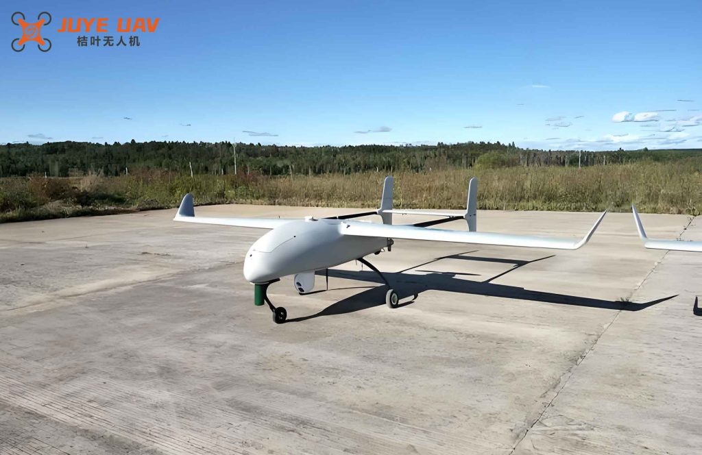
As an engineer working on flight control for small unmanned aerial vehicles, I have long been fascinated by the challenges posed by the fixed-wing drone. Unlike multi-rotor platforms, the fixed-wing drone exhibits strong coupling between longitudinal and lateral dynamics, a wide range of flight speeds, and severe sensitivity to wind gusts. The control of a fixed-wing drone must simultaneously regulate linear velocities (u, v, w), angular rates (p, q, r), and attitude angles (φ, θ, ψ). Traditional linear control methods such as PID are often insufficient when the fixed-wing drone operates far from the trim condition or under significant disturbances. This motivates me to explore advanced nonlinear control techniques that can handle the inherent multi-time-scale nature of the fixed-wing drone dynamics.
To this end, I adopt the singular perturbation theory, which is a powerful tool to analyze and control systems possessing both fast and slow dynamics. In the fixed-wing drone, the angular rate dynamics are inherently faster than the velocity and attitude dynamics. By introducing a small perturbation parameter ε, I can transform the full-order model into a standard singular perturbation form. Then, using time-scale decomposition, I obtain two reduced-order subsystems: a fast subsystem that governs the angular velocity response and a slow subsystem that governs the translational velocity and orientation. This decomposition greatly simplifies the controller design because each subsystem is of lower order and less coupled.
I begin by establishing the coordinate systems and the equations of motion for the fixed-wing drone in the body frame. Following the standard notation, let the body-fixed axes (x_e, y_e, z_e) be attached to the center of mass of the fixed-wing drone, with x_e pointing forward, y_e to the right, and z_e downward. The translational dynamics are given by Newton’s law in the body frame, and the rotational dynamics are given by Euler’s equation. The aerodynamic forces and moments are expressed as functions of the state vector and control inputs, using dimensionless coefficients obtained from wind tunnel experiments. The full nonlinear model of the fixed-wing drone can be written as:
$$
\begin{cases}
\dot{u} = r v – q w – g \sin\theta + \frac{1}{m} \left( \frac{1}{2}\rho V^2 S C_D + F_T \right) + D_{1u} \\
\dot{v} = p w – r u + g \cos\theta \sin\phi + \frac{1}{m} \left( \frac{1}{2}\rho V^2 S C_Y \right) + D_{1v} \\
\dot{w} = q u – p v + g \cos\theta \cos\phi + \frac{1}{m} \left( \frac{1}{2}\rho V^2 S C_L \right) + D_{1w} \\
\dot{p} = \frac{1}{I_{x_e}} \left[ (I_{y_e} – I_{z_e}) q r + J(\dot{r} + p q) + \frac{1}{2}\rho V^2 S b C_l \right] + D_{2p} \\
\dot{q} = \frac{1}{I_{y_e}} \left[ (I_{z_e} – I_{x_e}) p r + J(r^2 – p^2) + \frac{1}{2}\rho V^2 S b C_m + F_T Z_T \right] + D_{2q} \\
\dot{r} = \frac{1}{I_{z_e}} \left[ (I_{x_e} – I_{y_e}) p q + J(\dot{p} – q r) + \frac{1}{2}\rho V^2 S b C_n \right] + D_{2r} \\
\dot{\phi} = p + q \sin\phi \tan\theta + r \cos\phi \tan\theta \\
\dot{\theta} = q \cos\phi – r \sin\phi \\
\dot{\psi} = (q \sin\phi + r \cos\phi) \sec\theta
\end{cases}
$$
Here, u, v, w are the body-axis linear velocities; p, q, r are the angular rates; φ, θ, ψ are the Euler angles; m is the mass; I_xe, I_ye, I_ze are the moments of inertia; J is the product of inertia; ρ is the air density; V = sqrt(u²+v²+w²) is the total airspeed; S is the wing area; b is the wing span; F_T is the thrust; Z_T is the thrust moment arm; and D_{1u}, D_{1v}, D_{1w}, D_{2p}, D_{2q}, D_{2r} represent lumped disturbances (including external wind, unmodeled dynamics, etc.). The aerodynamic coefficients C_D, C_Y, C_L, C_l, C_m, C_n are functions of angle of attack α = arctan(w/u), sideslip angle β = arcsin(v/V), angular rates, and control surface deflections (elevator i_H, aileron δ_A, rudder δ_R, and throttle δ_T). Their expressions are given by linear aerodynamic models, e.g.,
$$
\begin{aligned}
C_D &= C_{D0} + C_{D\alpha} \alpha + C_{Dq} \frac{\bar{c}}{2V} q + C_{Di_H} i_H \\
C_L &= C_{L0} + C_{L\alpha} \alpha + C_{Lq} \frac{\bar{c}}{2V} q + C_{Li_H} i_H \\
C_m &= C_{m0} + C_{m\alpha} \alpha + C_{mq} \frac{\bar{c}}{2V} q + C_{mi_H} i_H \\
C_Y &= C_{Y0} + C_{Y\beta} \beta + C_{Yp} \frac{b}{2V} p + C_{Yr} \frac{b}{2V} r + C_{Y\delta_A} \delta_A + C_{Y\delta_R} \delta_R \\
C_l &= C_{l0} + C_{l\beta} \beta + C_{lp} \frac{b}{2V} p + C_{lr} \frac{b}{2V} r + C_{l\delta_A} \delta_A + C_{l\delta_R} \delta_R \\
C_n &= C_{n0} + C_{n\beta} \beta + C_{np} \frac{b}{2V} p + C_{nr} \frac{b}{2V} r + C_{n\delta_A} \delta_A + C_{n\delta_R} \delta_R
\end{aligned}
$$
The typical aerodynamic coefficients for the fixed-wing drone used in my simulation are listed in Table 1. These values are obtained from wind tunnel experiments on a 20.64 kg fixed-wing drone with a wingspan of 1.96 m and wing area of 1.37 m².
| Parameter | Value | Parameter | Value |
|---|---|---|---|
| CD0 | 0.072 | Cl0 | -0.007 |
| CDα | 0.382 | Clβ | -0.367 |
| CDq | 0 | Clp | -1.662 |
| CDiH | 0.145 | Clr | 0.145 |
| CL0 | 0 | ClδA | -0.505 |
| CLα | 6.947 | ClδR | 0.109 |
| CLq | 0 | Cn0 | 0.002 |
| CLiH | 1.517 | Cnβ | 0.109 |
| Cm0 | 0.045 | Cnp | -0.184 |
| Cmα | -0.707 | Cnr | -0.575 |
| Cmq | -1.713 | CnδA | -0.067 |
| CmiH | -0.543 | CnδR | -0.196 |
| CY0 | -0.022 | CYβ | 0.27 |
| CYp | 4.275 | CYr | -0.317 |
| CYδA | 1.017 | CYδR | -0.707 |
To apply singular perturbation, I partition the state vector into slow variables x = [u, v, w, φ, θ, ψ]ᵀ and fast variables z = [p, q, r]ᵀ. Notice that the aerodynamic moments depend on p, q, r, and the translational equations contain couplings from angular rates. After rearranging the equations, I obtain the following compact form:
$$
\begin{cases}
\dot{x} = f_1(x) z + f_2(x) + f_3(x) u + D_1(x,z,t) \\
\dot{z} = g_1(x) z + M_1 \dot{z} + g_2(x) + g_3(x) u + D_2(x,z,t)
\end{cases}
$$
where u is the control input vector (throttle, elevator, aileron, rudder). By isolating the term M₁ ż (which contains J), I solve for ż to get a standard state equation:
$$
\begin{cases}
\dot{x} = f_1(x) z + f_2(x) + f_3(x) u + D_1(x,z,t) \\
\dot{z} = G_1(x) z + G_2(x) + G_3(x) u + D_2(x,z,t)
\end{cases}
$$
where G₁(x) = (I − M₁)⁻¹ g₁(x), G₂(x) = (I − M₁)⁻¹ g₂(x), G₃(x) = (I − M₁)⁻¹ g₃(x). Now I introduce a small parameter ε (0 < ε ≪ 1) and define z = z₁/ε, so that:
$$
\begin{cases}
\dot{x} = F_1(x) z + f_2(x) + f_3(x) u + D_1(x,z,t) \\
\varepsilon \dot{z} = G(x) z + G_2(x) + G_3(x) u + D_2(x,z,t)
\end{cases}
$$
This is the singularly perturbed model of the fixed-wing drone. The parameter ε reflects the ratio of the time scales: the angular dynamics are ε times faster than the translational dynamics.
Setting ε = 0 yields the slow manifold equation:
$$
z_s = – G(x_s)^{-1} [ G_2(x_s) + G_3(x_s) u_s + D_2(x_s,z_s,t) ]
$$
Substituting into the slow dynamics gives the slow subsystem:
$$
\dot{x}_s = A(x_s) + U(x_s, u_s) + D_1(x_s,z_s,t)
$$
with A(x_s) = f₂(x_s) − F₁(x_s) G(x_s)⁻¹ G₂(x_s) and U(x_s,u_s) = [f₃(x_s) − F₁(x_s) G(x_s)⁻¹ G₃(x_s)] u_s.
For the fast subsystem, I define the fast time scale τ = t/ε and consider the deviation z_f = z − z_s, u_f = u − u_s. This leads to:
$$
\frac{d z_f}{d \tau} = G(x_s) z_f + G_3(x_s) u_f + D_2(x_s, z, t)
$$
Thus, the original system is decomposed into two lower-order subsystems: the slow subsystem (Eq. 8) governs the velocity and attitude dynamics, and the fast subsystem (Eq. 9) governs the angular rate dynamics. This decomposition allows me to design separate controllers for each loop, significantly reducing complexity.
Before designing the sliding mode controllers, I incorporate a nonlinear disturbance observer (NDO) to estimate the lumped disturbances D₁ and D₂. The disturbances are assumed to be bounded along with their first derivatives. For the slow subsystem, I design the NDO as:
$$
\begin{cases}
\hat{D}_1(x_s) = a_1 + Q_1(x_s) \\
\dot{a}_1 = – L_1(x_s) a_1 – L_1(x_s) ( Q_1(x_s) + A(x_s) + U )
\end{cases}
$$
where L₁(x_s) = ∂Q₁/∂x_s, and Q₁ is a chosen nonlinear gain vector. Similarly, for the fast subsystem, I design:
$$
\begin{cases}
\hat{D}_2(z_f) = a_2 + Q_2(z_f) \\
\dot{a}_2 = – L_2(z_f) a_2 – L_2(z_f) ( G(x_s) z_f + G_3(x_s) u_f )
\end{cases}
$$
I choose Q₁ and Q₂ such that the estimation errors e_NDO₁ = D₁ − \hat{D}_₁ and e_NDO₂ = D₂ − \hat{D}_₂ converge to a small residual bound. The convergence analysis shows that by selecting Lipschitz gains, the estimation error can be made arbitrarily small. For my design, I set Q₁(x_s) = diag{ 5(u + u³/3), 5(v + v³/3), 5(w + w³/3), 15(φ + φ³/3), 15(θ + θ³/3), 15(ψ + ψ³/3) }.
Now I present the sliding mode control design. For the slow subsystem, define the tracking error X_e = X_c − X_s, where X_c is the commanded velocity and attitude vector. The sliding surface is S_s = C_s X_e with C_s = diag{1,1,1,1,1,1}. The control law is derived by setting Ṡ_s = 0 and incorporating the disturbance estimate:
$$
U = C_s^{-1} [ C_s \dot{x}_c – C_s A(x_s) – C_s \hat{D}_1 – K_1 S_s – \hat{\beta}_{d1} \tanh(S_s) ]
$$
where K₁ > 0 is a gain matrix, and \hat{β}_{d1} is an adaptive gain updated by \dot{\hat{β}}_{d1} = ‖C_s‖ ‖S_s‖. The tanh function smooths the switching control, effectively eliminating chattering. Lyapunov analysis shows that V = ½ S_sᵀ S_s + (1/(2λ)) β_e², with β_e = β_d − \hat{β}_{d1}, has a negative semidefinite derivative, ensuring asymptotic convergence of tracking errors.
For the fast subsystem, define the angular rate error z_e = z_c − z_f, and the sliding surface S_f = C_f z_e with C_f = diag{1,1,1}. The composite control law (including the disturbance estimate) is:
$$
u_f = \varepsilon (C_f G_3(x_s))^{-1} [ C_f \dot{z}_c – C_f G(x_s) z_f – C_f \hat{D}_2 – K_2 S_f – \hat{\beta}_{d2} \tanh(|S_f|) ]
$$
with adaptive law \dot{\hat{β}}_{d2} = ‖C_f‖ ‖S_f‖. Again, Lyapunov stability is guaranteed for K₂ > 0.
I have implemented the full control system in Simulink for a fixed-wing drone model with the parameters given in Table 1. The mass m = 20.64 kg, wing span b = 1.96 m, wing area S = 1.37 m², moments of inertia I_xe = 1.6073 kg·m², I_ye = 7.5085 kg·m², I_ze = 7.1865 kg·m², product of inertia J = -0.561 kg·m². The commanded signals are piecewise constant functions: for the slow states, X_c = [40H(t)−20, 10H(t)−5, 10H(t)−5, 2H(t)−1, 2H(t)−1, 2H(t)−1]ᵀ, where H(t) is a periodic step function with period 10 s (50% duty cycle). For the angular rates, z_c = [2H(t)−1, 2H(t)−1, 2H(t)−1]ᵀ. External disturbances are injected as D₁ = [10 sin(t), 10 sin(t), 10 sin(t), sin(t), sin(t), sin(t)]ᵀ and corresponding D₂.
Two key simulation cases are compared: (1) with the proposed disturbance observer-based sliding mode control (DOB-SMC) after singular perturbation decomposition, and (2) without the disturbance observer (i.e., standard sliding mode control on the decoupled subsystems). The results demonstrate that the DOB-SMC achieves much faster convergence and smaller steady-state errors. Specifically, the slow subsystem responses show that the linear velocities u, v, w and Euler angles φ, θ, ψ track the desired commands accurately, with negligible overshoot. In contrast, the standard SMC without disturbance observer exhibits noticeable oscillations and steady-state biases due to the uncompensated disturbances. The fast subsystem responses (p, q, r) also show superior tracking performance with DOB-SMC. The chattering phenomenon is effectively mitigated by the tanh function, as evident from the smooth control signals.
Furthermore, I compare the performance of the singular-perturbation-based decoupled control with a conventional “full-order” sliding mode controller that does not exploit the time-scale separation. The decoupled control yields faster response in the fast loop because the fast subsystem controller operates in the fast time scale τ, effectively increasing the bandwidth. This is particularly beneficial for the fixed-wing drone, where rapid angular rate stabilization is critical for maneuverability and disturbance rejection.
In conclusion, the singular perturbation decomposition combined with the disturbance observer-based adaptive sliding mode control provides an effective solution for high-precision flight control of a fixed-wing drone. The key contributions of this work are: (1) establishing a singularly perturbed model for the fixed-wing drone dynamics, (2) applying time-scale decomposition to decouple the fast angular rate loop from the slow velocity/attitude loop, (3) designing nonlinear disturbance observers to estimate internal and external disturbances, and (4) developing adaptive sliding mode controllers with tanh switching to eliminate chattering. Simulation results validate the approach, showing significant improvement in tracking accuracy and disturbance rejection over conventional methods. Future work will focus on extending the method to formation flight and adaptive control under varying mass and aerodynamic parameters.