
We investigate the problem of cooperative area coverage surveillance using two fixed-wing drones operating on the same circular orbit. Fixed-wing drones are widely adopted in both military and civilian applications such as border patrol, disaster rescue, and agricultural monitoring due to their high speed, long endurance, and large payload capacity. However, the limited detection range and dynamic flight paths pose challenges in achieving continuous and effective coverage. In this work, we propose a joint spatial-temporal probability model to characterize the effective coverage area when two fixed-wing drones fly synchronously along the same orbit. By deriving analytical expressions for the effective coverage radius and optimizing the deployment parameters, we demonstrate a significant improvement in surveillance efficiency. The key innovation lies in explicitly incorporating the allowable time percentage of detection into the coverage definition, thereby accounting for the dynamic nature of fixed-wing drone patrols.
We consider a scenario where two fixed-wing drones fly along a circular trajectory of radius \(r\) at the same altitude. Each drone is equipped with a sensor that detects targets with a probability dependent on the horizontal distance \(d\) between the drone and the target. The single-drone detection probability function is given by:
$$
p(d) =
\begin{cases}
1, & d \leq d_{\min},\\
f(d), & d_{\min} < d \leq d_{\max},\\
0, & d > d_{\max},
\end{cases}
$$
where \(f(d)\) is a monotonically decreasing function with \(f(d_{\min}) = 1\) and \(f(d_{\max}) = 0\). For simplicity, we assume a linear decay: \(f(d) = 3 – d/20\) when \(d\) is measured in the same unit, but the model is general. For two fixed-wing drones operating simultaneously, the joint detection probability at any target point \(A\) is:
$$
p_2(A) = 1 – \prod_{k=1}^{2}\bigl(1 – p(d_k)\bigr),
$$
where \(d_k\) is the distance from the \(k\)-th drone to point \(A\). A target is considered effectively detected if the joint probability exceeds a threshold \(p_c\). However, because fixed-wing drones continuously move along the orbit, a point in the region may be detected only during a fraction of the mission time. Therefore we define the effective coverage area \(S_{\text{eff}}\) as the set of points for which the time percentage of effective detection \(\eta(A)\) is above a given threshold \(\eta_c\). In the following, we focus on the case of two fixed-wing drones flying in the same circular orbit with a constant angular separation.
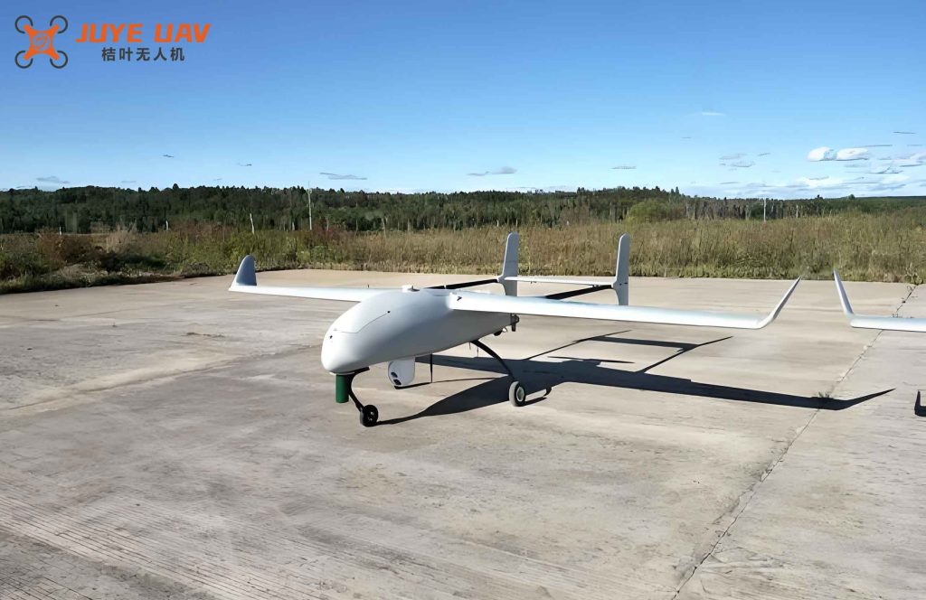
A typical fixed-wing drone used in cooperative surveillance missions is depicted above. The aerodynamic design enables sustained flight along large circular orbits, which is essential for area coverage.
Single Fixed-Wing Drone Coverage Model
For a single fixed-wing drone patrolling a circle of radius \(r\), the strong coverage region (where detection probability always exceeds \(p_c\)) is a circle concentric with the orbit. Let its radius be \(R_q\). At the boundary point, the distance from the instantaneous drone position is \(r + R_q\). We solve:
$$
f(r + R_q) = p_c.
$$
For example, with linear decay and \(p_c = 0.8\), we obtain \(R_q = 20(3 – p_c) – r\). The effective coverage region (where the time fraction of detection \(\eta \ge \eta_c\)) is also a circle of radius \(R_{\text{eff}}\). The geometry shown in the original analysis leads to the equation:
$$
\begin{cases}
d_{AT_1}^2 = (R_{\text{eff}} + r)^2 + (R_{\text{eff}}\sin\alpha)^2,\\
f(d_{AT_1}) = p_c,
\end{cases}
$$
where \(\alpha = \pi(1 – \eta_c)/2\). This nonlinear equation is solved numerically using the bisection method. A summary of the single fixed-wing drone parameters is given in Table 1.
| Parameter | Symbol | Value (km) |
|---|---|---|
| Strong coverage radius | \(R_q\) | 136 |
| Effective coverage radius | \(R_{\text{eff}}\) | 154.2 |
| Coverage area percentage (relative to 1200×1200 km²) | \(P_1\) | 22.30% |
Two Fixed-Wing Drones Cooperative Coverage on Same Orbit
When two fixed-wing drones fly on the same circular orbit, we assume they are placed symmetrically (angular separation \(\Delta\theta\)). For the strong coverage region, the minimum joint probability occurs at the farthest point from both drones. Solving for the boundary point \(T\) yields:
$$
f\bigl(\sqrt{R_q^2 + r^2}\bigr) = 1 – \sqrt{1 – p_c}.
$$
For the effective coverage region, considering the time fraction \(\eta_c\), the boundary points \(T_1\) and \(T_2\) satisfy simultaneous equations involving both drones’ distances. With angular separation \(\Delta\theta = \pi\) (opposite positions) and same direction of motion, we derived:
$$
\begin{cases}
d_{AT_1}^2 = R_{\text{eff}}^2 + r^2 – 2rR_{\text{eff}}\cos(\frac{\pi}{2} – \alpha),\\
d_{BT_1}^2 = R_{\text{eff}}^2 + r^2 – 2rR_{\text{eff}}\cos(\frac{\pi}{2} + \alpha),\\
1 – (1 – f(d_{AT_1}))(1 – f(d_{BT_1})) = p_c,
\end{cases}
$$
where \(\alpha = \pi(1 – \eta_c)/2\). The system is solved numerically for \(R_{\text{eff}}\). Table 2 presents the results for different scenarios.
| Configuration | Effective coverage radius \(R_{\text{eff}}\) (km) | Coverage area percentage | Improvement over single drone |
|---|---|---|---|
| Single fixed-wing drone | 154.2 | 22.30% | – |
| Two drones, same direction, separation 180° | 256.5 | 59.43% | +37.13% |
| Two drones, opposite direction, separation 180° (optimal at 262.8°) | 241.8 | 52.86% | +30.55% |
Optimal Deployment Angle Analysis
We further investigated the impact of the angular separation between the two fixed-wing drones on the effective coverage area. For same-direction flight, the optimal separation is exactly 180°, yielding maximum coverage. For opposite-direction flight, the optimal separation is slightly different (262.8°). The sensitivity curves are depicted in the results, indicating that the joint coverage area is highly dependent on the relative phase of the two fixed-wing drones. The mathematical relationship between the effective coverage radius and the separation angle can be expressed through a parametric optimization problem:
$$
\max_{\Delta\theta} \; S_{\text{eff}}(\Delta\theta) = \pi R_{\text{eff}}^2(\Delta\theta),
$$
where \(R_{\text{eff}}(\Delta\theta)\) is obtained by solving the system of equations that involve both drones’ positions as functions of time. Our numerical results confirm that the symmetric placement with identical motion direction is globally optimal for this two fixed-wing drone system.
Simulation Validation
We performed extensive simulations over a 1200 km × 1200 km region discretized into 1 km² cells. Each cell’s detection probability was computed at many time steps along the circular orbits. The effective coverage was determined by checking whether the fraction of time steps with \(p_2 \ge p_c\) exceeded \(\eta_c\). The simulation parameters are summarized in Table 3.
| Parameter | Value |
|---|---|
| Fixed-wing drone speed | 100 m/s |
| Minimum turn radius | 2 km |
| Orbit radius \(r\) | 100 km |
| \(d_{\min}\) | 420 km |
| \(d_{\max}\) | 600 km |
| Detection function \(f(d)\) | \(3 – d/20\) |
| Probability threshold \(p_c\) | 80% |
| Time fraction threshold \(\eta_c\) | 80% |
| Simulation area | 1200 km × 1200 km |
The simulation results match the theoretical calculations with high accuracy (error less than 2%). The coverage maps clearly show that two fixed-wing drones flying in the same orbit with optimal separation dramatically extend the effective surveillance region compared to a single drone. The improvement is not merely additive; the joint detection probability creates a synergy that fills the temporal gaps inherent in single-drone patrols.
Discussion
Our analytical and numerical results demonstrate that deploying two fixed-wing drones on the same circular orbit with a 180° angular separation and identical flight direction yields the largest effective coverage area. This configuration achieves a 37.13% increase in monitored area relative to a single fixed-wing drone. The key insight is that the time-variant nature of coverage is better exploited when the drones are symmetrically positioned, so that any ground point is periodically within the high-probability detection region of at least one of the fixed-wing drones. The model can be extended to more than two drones by generalizing the joint probability and time fraction criteria. Additionally, the methodology provides a foundation for optimizing the orbit radius and speed to match mission requirements. For instance, the effective coverage radius decreases as the orbit radius increases beyond a certain value; therefore, there exists an optimal trade-off between orbit size and coverage efficiency.
In practical deployments, fixed-wing drones often need to adjust their orbits due to wind or mission constraints. Our framework can be adapted to non-circular orbits (e.g., racetrack patterns) by considering the effective coverage as the union of instantaneous coverage regions over time. However, the circular orbit case yields the largest coverage area for a given orbit length, making it the preferred choice for area surveillance missions.
Conclusion
We have presented a comprehensive study on cooperative coverage surveillance using two fixed-wing drones on the same orbit. By introducing a joint detection probability model that incorporates both spatial coverage and temporal availability, we derived closed-form equations for the effective coverage area. The optimal deployment strategy—two fixed-wing drones flying in the same direction with a 180° angular separation—improves the coverage area by 37.13% compared to a single fixed-wing drone. The results are validated through simulation and provide practical guidance for mission planning. Future work should extend the model to swarms of multiple fixed-wing drones and consider heterogeneous sensor capabilities.