
In recent years, as drone technology has matured, Unmanned Aerial Systems (UAS) have been increasingly applied from military to civilian domains. When large-scale communication infrastructure is paralyzed by disasters, medium-altitude vertical takeoff and landing fixed-wing drones can quickly fly to designated locations and provide wireless network coverage to ground terminals using onboard emergency equipment. In-depth investigation of air-to-ground channel models and characteristics under emergency scenarios is of great significance for the design and optimization of UAS communication systems. In 2017, 3GPP initiated the study of LTE aerial channels and developed several protocol specifications, but they only focus on low-altitude wireless communication below 300 m for terrestrial mobile terminals. Traditional channel models such as Okumura-Hata and Uma are also only applicable to ground scenarios. Akram Al-Hourani et al. studied the air-to-ground path loss model in urban environments, but that model only applies to static base station transmission and is not suitable for medium- and low-altitude, highly dynamic fixed-wing drone emergency scenarios. All the above models target small drones at low altitudes and are not applicable to the emergency scenarios of medium- and high-altitude, highly dynamic medium-to-large fixed-wing drones. Moreover, those models are based on traditional empirical models and have low applicability and accuracy in practical use. Based on the machine learning XGBoost algorithm, we propose an air-to-ground intelligent propagation model specifically for medium-sized fixed-wing drone emergency scenarios. By extracting features from engineering parameter data collected by aerial base stations, we innovatively incorporate dynamic 3D antenna gain values to improve prediction accuracy. We compare our model with traditional air-to-ground channel models and the channel model proposed in 3GPP 36.777. Results show that the XGBoost-based path loss model achieves significantly higher prediction accuracy compared to traditional wireless propagation models.
Experimental System Setup and Feature Preprocessing
System Setup
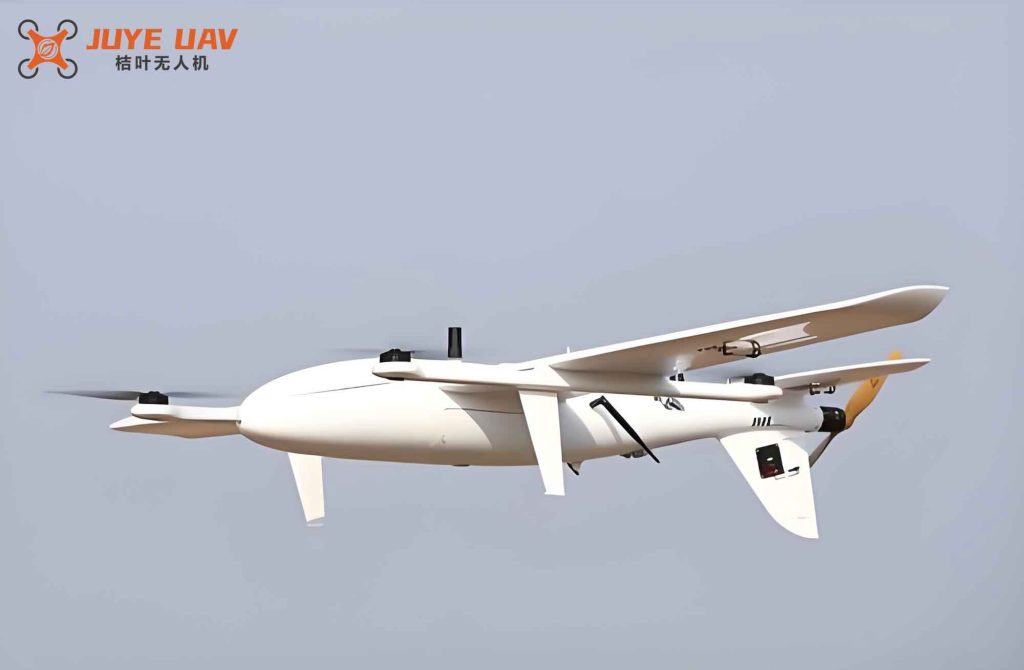
The field tests were conducted in open areas. The ground receiving terminal was approximately 1 m high. An aerial drone equipped with a base station and antenna transmitted signals at a working frequency of 900 MHz. The ground terminal recorded the received signal strength and its own position. The drone’s position, attitude, and other relevant information were stored in the drone control terminal for subsequent data analysis. The test base station was a commercial LTE FDD 900M system. The 900 MHz band has strong diffraction capability in free space and suffers less fading. The onboard antenna operated in the 820–960 MHz band with a maximum gain of 3 dBi. The antenna was suspended on the wing side of the fixed-wing drone to achieve continuous coverage. During flight tests, the drone flew clockwise in a circle with a radius of 300 m. The drone flew at altitudes of 500 m, 1000 m, and 1500 m respectively. Test personnel started from the center of the circle and performed fixed-point and distance-extension tests every 0.5 km.
Feature Construction
The experimental data included 12 original features such as drone (base station) position, terminal position, signal transmission power, and drone flight attitude. A total of 8000 data samples were collected. After preprocessing, 7 constructed features related to geometry and angles were added, as summarized in Table 1.
| Feature Type | Original Features | Constructed Features | Unit |
|---|---|---|---|
| Geometric | Receiver longitude \(A_j\) | Horizontal distance \(d_{2D}\) | m |
| Receiver latitude \(A_w\) | 3D distance \(d_{3D}\) | m | |
| Drone longitude \(B_j\) | Height difference \(H_d\) | m | |
| Drone latitude \(B_w\) | – | – | |
| Terminal height \(H_{ue}\) | – | – | |
| Angular | Drone altitude \(H_{uav}\) | Azimuth of terminal relative to drone \(\phi_{ue}\) | rad |
| Drone speed \(V_{uav}\) | Elevation of terminal relative to drone \(\theta_{ue}\) | rad | |
| Drone heading \(\phi_{uav}\) | Azimuth of terminal relative to antenna \(\phi\) | rad | |
| Channel | Drone roll \(\theta_{uav}\) | Elevation of terminal relative to antenna \(\theta\) | rad |
| Transmit power \(P_{Tx}\) | – | MHz | |
| Carrier frequency \(f_c\) | – | MHz | |
| – | 3D antenna gain \(G_{Tx3D}\) | – | dBi |
Distance and Angle Feature Construction
Assume the horizontal distance between the drone base station and the ground terminal is \(d_{2D}\). Let \(A\) denote the terminal location and \(B\) the drone location. \(R\) is the Earth’s mean radius. Let \(A_j, A_w\) be the longitude and latitude of the terminal, and \(B_j, B_w\) those of the drone. The angle \(c\) subtended by the great circle arc \(AB\) is computed from the spherical cosine law:
\[
c = \arccos\left( \cos(90^\circ – B_w)\cos(90^\circ – A_w) + \sin(90^\circ – B_w)\sin(90^\circ – A_w)\cos(B_j – A_j) \right)
\]
Converting to radians:
\[
c(\text{rad}) = \frac{c\pi}{180}
\]
Then the horizontal distance and 3D distance are:
\[
d_{2D} = R \cdot c
\]
\[
d_{3D} = \sqrt{d_{2D}^2 + (H_{uav} – H_{ue})^2}
\]
where \(H_{ue}\) is the terminal height and \(H_{uav}\) is the drone altitude.
The azimuth of the terminal relative to the drone, \(\phi_{ue}\), measured clockwise from true north, is derived from the spherical triangle:
\[
\phi_{ue} = \arctan\left( \frac{(B_j – A_j)\cos B_w}{B_w – A_w} \right)
\]
The elevation angle \(\theta_{ue}\) (angle between the line connecting terminal and drone and the horizontal plane) is:
\[
\theta_{ue} = \arctan\left( \frac{d_{2D}}{H_{uav} – H_{ue}} \right)
\]
Dynamic 3D Antenna Gain Construction
During actual measurements, the positions of the terminal and drone change dynamically, so the antenna gain at each point is a dynamic 3D gain rather than a fixed value. We innovatively applied dynamic 3D antenna gain in the air-to-ground propagation model to reduce the error caused by antenna gain on path loss. The antenna gain was simulated using interpolation based on the measured E-plane and H-plane radiation patterns. The interpolation formula is:
\[
Gain(\Phi_s, \theta_s) = H(\Phi_s) – \left[ \frac{\pi – |\Phi_s|}{\pi} (H(0) – V(\theta_s)) + \frac{|\Phi_s|}{\pi} (H(\pi) – V(\pi – \theta_s)) \right]
\]
Here, \(\Phi_s\) is the horizontal angle of the terminal in the drone coordinate system, and \(\theta_s\) is the elevation angle. \(H(\Phi_s)\) and \(V(\theta_s)\) are the horizontal and vertical gains at those angles, respectively. The azimuth \(\phi\) and elevation \(\theta\) of the terminal relative to the 3D antenna are obtained by subtracting the drone’s roll and heading angles from the relative angles and taking modulo \(2\pi\):
\[
\phi = (\phi_{ue} – \phi_{uav}) \mod (2\pi)
\]
\[
\theta = (\theta_{ue} – \theta_{uav}) \mod (2\pi)
\]
Using the computed \(\phi\) and \(\theta\), we looked up the simulated 3D antenna gain value \(G_{Tx3D}\). The measured path loss \(PL\) is then derived from the link budget equation:
\[
PL = P_{Tx} + G_{Tx3D} + G_{rx} – P_{Rx}
\]
where \(P_{Tx}\) is the transmit power, \(G_{rx}\) is the receiver antenna gain, and \(P_{Rx}\) is the measured received power.
Feature Selection
To evaluate the influence of each feature on path loss, we computed the Pearson correlation coefficient between each feature vector and \(PL\). The Pearson coefficient is defined as:
\[
\rho_{XY} = \frac{\text{cov}(X,Y)}{\sigma_X \sigma_Y} = \frac{E[(X – \mu_X)(Y – \mu_Y)]}{\sigma_X \sigma_Y}
\]
where \(X\) is the feature vector, \(Y\) is the path loss, \(\mu_X, \mu_Y\) are means, and \(\sigma_X, \sigma_Y\) are standard deviations. The correlation results sorted by absolute value are shown in Table 2.
| Rank | Feature | Correlation | |Correlation| |
|---|---|---|---|
| 1 | \(d_{3D}\) | 0.29 | 0.29 |
| 2 | \(d_{2D}\) | 0.28 | 0.28 |
| 3 | \(\theta_{ue}\) | -0.28 | 0.28 |
| 4 | \(\theta_{uav}\) | -0.26 | 0.26 |
| 5 | \(\phi_{ue}\) | 0.21 | 0.21 |
| 6 | \(V_{uav}\) | -0.2 | 0.2 |
| 7 | \(\phi_{uav}\) | 0.18 | 0.18 |
| 8 | \(H_d\) | -0.13 | 0.13 |
Path loss is most strongly correlated with \(d_{3D}\), \(d_{2D}\), \(\theta_{ue}\), \(\theta_{uav}\), and \(\phi_{ue}\). Therefore, we selected these five features \(\{d_{3D}, d_{2D}, \theta_{ue}, \theta_{uav}, \phi_{ue}\}\) as input vectors for constructing the propagation model.
Classic Path Loss Models
Evaluation Metrics
We used the root mean square error (RMSE) and mean error (ME) to evaluate model performance. For \(n\) samples:
\[
\text{RMSE} = \sqrt{\frac{1}{n} \sum_{i=1}^n (y_i – \hat{y}_i)^2}
\]
\[
\text{ME} = \frac{1}{n} \sum_{i=1}^n (y_i – \hat{y}_i)
\]
where \(y_i\) is the measured path loss and \(\hat{y}_i\) is the predicted path loss for the \(i\)-th sample.
3GPP Model
In 3GPP TR 36.777, the RMa-AV LOS model is defined for low-altitude (below 300 m) air-to-ground scenarios. The model is:
\[
PL_{\text{3GPP}}^{\text{RMa-AV-LOS}}(f_c, d_{3D}) = \max(23.9 – 1.8\log_{10}(H_{uav}), 20) \log_{10}(d_{3D}) + 20\log_{10}\left(\frac{40\pi f_c}{3}\right)
\]
with conditions \(10\text{ m} \le H_{uav} \le 300\text{ m}\) and \(d_{2D} \le 10\text{ km}\). For medium-to-high altitudes, this model effectively reduces to the free-space path loss model:
\[
PL = 20\log_{10}(d) + 20\log_{10}(f) + 20\log_{10}\left(\frac{4\pi}{c}\right)
\]
A2G Model
The air-to-ground (A2G) path loss model proposed by Akram Al-Hourani et al. accounts for line-of-sight (LOS) and non-line-of-sight (NLOS) probabilities. The signal in high altitude experiences free-space propagation; at very low altitudes it may be obstructed by ground obstacles. The LOS and NLOS path losses are:
\[
PL_{\text{LOS}} = 20\log_{10}(d) + 20\log_{10}(f) + 20\log_{10}\left(\frac{4\pi}{c}\right) + \eta_{\text{LOS}}
\]
\[
PL_{\text{NLOS}} = 20\log_{10}(d) + 20\log_{10}(f) + 20\log_{10}\left(\frac{4\pi}{c}\right) + \eta_{\text{NLOS}}
\]
where \(\eta_{\text{LOS}}\) and \(\eta_{\text{NLOS}}\) are excess losses depending on the environment. The average path loss is:
\[
PL = P_{\text{LOS}} \cdot PL_{\text{LOS}} + P_{\text{NLOS}} \cdot PL_{\text{NLOS}}
\]
The LOS probability is given by the ITU-R model and fitted as:
\[
P_{\text{LOS}} = \frac{1}{1 + a e^{-b\left(\frac{180}{\pi}\theta – a\right)}}
\]
where \(a\) and \(b\) are environment-dependent parameters, and \(\theta\) is the elevation angle. The final consolidated A2G model becomes:
\[
PL = \frac{\eta_{\text{LOS}} – \eta_{\text{NLOS}}}{1 + a e^{-b(\theta – a)}} + 20\log_{10}(d) + 20\log_{10}(f) + 20\log_{10}\left(\frac{4\pi}{c}\right) + \eta_{\text{NLOS}}
\]
XGBoost-Based Wireless Channel Model
XGBoost (eXtreme Gradient Boosting) is an efficient implementation of gradient boosted decision trees, known for high prediction accuracy. We adopted XGBoost as the core algorithm for path loss inversion in the highly dynamic fixed-wing drone emergency scenario. The key steps are summarized below.
Regularized Loss Function
The objective function consists of training loss and a regularization term to prevent overfitting:
\[
\text{Loss}(\mathbf{x}_i) = \sum_{i=1}^n l(\hat{y}_i, y_i) + \sum_{i=1}^t \Omega(f_i)
\]
\[
\Omega(f) = \gamma T + \frac{1}{2}\lambda \sum_{j=1}^T \omega_j^2
\]
Here, \(\gamma T\) penalizes the number of leaves, and \(\frac{1}{2}\lambda \sum \omega_j^2\) penalizes leaf weights. The tree model is \(f_t(x) = w_{q(x)}\), where \(q(x)\) maps input features to leaf indices. Our input features for each sample \(i\) are \(\{d_{3D,i}, d_{2D,i}, \theta_{ue,i}, \theta_{uav,i}, \phi_{ue,i}\}\).
Additive Training and Taylor Expansion
At the \(t\)-th iteration, the prediction is updated as \(\hat{y}_i^{(t)} = \hat{y}_i^{(t-1)} + f_t(\mathbf{x}_i)\). The objective becomes:
\[
\text{Loss}^{(t)} = \sum_{i=1}^n l\big(y_i, \hat{y}_i^{(t-1)} + f_t(\mathbf{x}_i)\big) + \sum_{i=1}^{t-1} \Omega(f_i) + \Omega(f_t)
\]
We expand the loss to second order using Taylor series around \(\hat{y}_i^{(t-1)}\):
\[
\text{Loss}^{(t)} \approx \sum_{i=1}^n \left[ l(y_i,\hat{y}_i^{(t-1)}) + g_i f_t(\mathbf{x}_i) + \frac{1}{2} h_i f_t^2(\mathbf{x}_i) \right] + \sum_{i=1}^{t-1} \Omega(f_i) + \Omega(f_t)
\]
where \(g_i = \partial_{\hat{y}^{(t-1)}} l(y_i, \hat{y}_i^{(t-1)})\) and \(h_i = \partial^2_{\hat{y}^{(t-1)}} l(y_i, \hat{y}_i^{(t-1)})\). Removing constant terms and substituting the tree model and regularization yields:
\[
\text{Loss}^{(t)} \approx \sum_{i=1}^n \left[ g_i w_{q(\mathbf{x}_i)} + \frac{1}{2} h_i w_{q(\mathbf{x}_i)}^2 \right] + \gamma T + \frac{1}{2}\lambda \sum_{j=1}^T w_j^2
\]
Optimal Leaf Weights
Define the set of samples in leaf \(j\) as \(I_j = \{i | q(\mathbf{x}_i) = j\}\). Then:
\[
\text{Loss}^{(t)} \approx \sum_{j=1}^T \left[ \left(\sum_{i \in I_j} g_i\right) w_j + \frac{1}{2} \left(\sum_{i \in I_j} h_i + \lambda\right) w_j^2 \right] + \gamma T
\]
The optimal leaf weight \(w_j^*\) that minimizes the loss is given by setting the derivative to zero:
\[
w_j^* = – \frac{G_j}{H_j + \lambda}
\]
where \(G_j = \sum_{i \in I_j} g_i\) and \(H_j = \sum_{i \in I_j} h_i\). The minimal loss becomes:
\[
\text{Loss}^* = -\frac{1}{2} \sum_{j=1}^T \frac{G_j^2}{H_j + \lambda} + \gamma T
\]
Split Gain
When splitting a leaf into left and right child nodes, the gain is computed as:
\[
\text{Gain} = \frac{1}{2} \left[ \frac{G_L^2}{H_L + \lambda} + \frac{G_R^2}{H_R + \lambda} – \frac{(G_L+G_R)^2}{(H_L+H_R) + \lambda} \right] – \gamma
\]
The split point that yields the largest gain is selected. The greedy exact algorithm iterates over all possible split values for each feature to find the best split. The algorithm for our five features is described in Table 3.
| Input | Current node dataset with features \(\{d_{3D}, d_{2D}, \theta_{ue}, \theta_{uav}, \phi_{ue}\}\) and target \(PL\). Feature dimension \(m=5\). |
|---|---|
| Initialize | \(G = \sum_{i \in I} g_i\), \(H = \sum_{i \in I} h_i\) for the current node. |
| For each feature \(k=1..m\) | Sort the instances by feature value. Initialize \(G_L=0, H_L=0\). For each sorted instance: update \(G_L\) and \(H_L\), then compute \(G_R = G – G_L\), \(H_R = H – H_L\), and score \(\frac{G_L^2}{H_L+\lambda} + \frac{G_R^2}{H_R+\lambda} – \frac{G^2}{H+\lambda}\). Keep the maximum score. |
| Output | Split point with maximum gain. |
Experimental Results and Analysis
To validate the accuracy of the XGBoost-based intelligent propagation model for fixed-wing drone scenarios, we compared it with the classical 3GPP RMa-AV LOS model and the A2G model. All models used the same training and testing datasets collected from field tests at two different open-area sites. The XGBoost model was optimized via grid search; the final hyperparameters are listed in Table 4.
| Parameter | Value |
|---|---|
| Maximum depth | 6 |
| Learning rate | 0.1 |
| Number of boosting rounds | 1000 |
| Booster | gbtree |
| Gamma | 0 |
| Lambda | 3 |
| Objective | logistic |
| Subsample ratio | 0.7 |
Results from both test sites show that the path loss varies significantly as the fixed-wing drone circles, with fluctuations up to about 20 dB. The XGBoost model captures these dynamic changes much better than the classical models. The classical models only fit the average trend, while XGBoost accurately predicts path loss at each location. Tables 5 and 6 present the error metrics for both sites.
| Model | RMSE (dB) | ME (dB) |
|---|---|---|
| 3GPP | 10.60 | 12.93 |
| A2G | 10.28 | 12.77 |
| XGBoost | 3.64 | -0.80 |
| Model | RMSE (dB) | ME (dB) |
|---|---|---|
| 3GPP | 7.86 | 9.95 |
| A2G | 7.20 | 9.23 |
| XGBoost | 4.99 | -0.15 |
The XGBoost model achieves RMSE values of 3.64 dB and 4.99 dB at the two sites, which are much lower than those of the 3GPP and A2G models. The mean error is close to zero (–0.80 dB and –0.15 dB), indicating unbiased predictions. The classical models show significantly larger errors, especially in the mean error, because they cannot track the rapid fluctuations caused by the fixed-wing drone’s attitude changes. The CDF curves of RSRP also confirm that the XGBoost model’s distribution closely matches the measured data.
Conclusion
We built an air-to-ground intelligent propagation model based on the XGBoost algorithm specifically for medium-to-high altitude fixed-wing drone emergency scenarios. Innovatively, we incorporated dynamic 3D antenna gain values into the feature set. The proposed model was compared with the classic 3GPP RMa-AV LOS model and the A2G model using real field test data. The results demonstrate that the XGBoost model significantly outperforms the classical models in prediction accuracy, with RMSE below 5 dB and mean error close to zero. This high accuracy is crucial for precise air-to-ground channel path loss prediction in highly dynamic emergency scenarios involving fixed-wing drones.