
In the realm of autonomous flight, the ability of a fixed-wing drone to maintain stable and accurate control under severe wind disturbances remains a critical challenge. Traditional nonlinear dynamic inversion (NDI) control methods rely heavily on the fidelity of the aerodynamic model. However, in real-world scenarios, especially under strong and time-varying wind conditions, the aerodynamic forces and moments acting on a fixed-wing drone can deviate significantly from pre-computed models. To address this issue, we have developed an adaptive dynamic inverse flight control law that integrates meta-learning flight concepts with real-time aerodynamic modeling. This approach enables the fixed-wing drone to continuously learn from its own flight states and adapt its control commands accordingly.
The core idea is to combine a neural network-based common basis function model, which captures the inherent aerodynamic characteristics of the aircraft, with a Kalman filter that estimates the wind interference coefficients online. This synergy allows the fixed-wing drone to predict its aerodynamic forces and moments in real time, even under unknown and varying wind fields. The dynamic inversion control framework is then designed with three nested loops: a fast loop for angular rates, a medium loop for attitude angles, and a slow loop for translational velocity. A particular difficulty arises in the velocity loop due to the non-affine relationship between acceleration and attitude angles. We employ a Taylor expansion to linearize this relationship, transforming it into an affine form that can be inverted directly.
This paper presents a comprehensive study of the proposed method, including detailed mathematical derivations, a description of the online learning mechanism, and extensive simulation validations under both time-varying wind and wind shear conditions. The results demonstrate that the adaptive dynamic inverse controller significantly improves the tracking performance and robustness of the fixed-wing drone in harsh environments. The following sections elaborate on the methodology, the control architecture, and the simulation outcomes.
Methodology
Real-Time Aerodynamic Modeling via Meta-Learning
The foundation of our adaptive control lies in the real-time aerodynamic model. Based on the Chebyshev polynomial expansion theory, we represent the aerodynamic forces and moments of the fixed-wing drone as the product of a common basis function matrix Ψ(x) (dependent only on the aircraft’s own motion states) and a wind interference coefficient vector a(ω̃) (dependent only on the wind velocity vector). The relationship is expressed as:
$$
\begin{bmatrix} F_X \\ F_Y \\ F_Z \\ M_X \\ M_Y \\ M_Z \end{bmatrix} \approx \Psi(\mathbf{x}) \begin{bmatrix} a_{F_X}(\tilde{\omega}) \\ a_{F_Y}(\tilde{\omega}) \\ a_{F_Z}(\tilde{\omega}) \\ a_{M_X}(\tilde{\omega}) \\ a_{M_Y}(\tilde{\omega}) \\ a_{M_Z}(\tilde{\omega}) \end{bmatrix}
$$
where x includes the quaternion, body-axis velocities, angular velocities, and control surface deflections of the fixed-wing drone. The common basis function neural network is pre-trained offline using flight data from a wide range of maneuvers under calm conditions. This network encodes the inherent aerodynamic characteristics of the aircraft, such as its stability derivatives and control effectiveness. During real-time flight, we only need to estimate the six wind coefficients a = [a_{F_X}, a_{F_Y}, a_{F_Z}, a_{M_X}, a_{M_Y}, a_{M_Z}]^T. To achieve this, we treat the wind coefficients as slowly varying parameters and augment them into the state vector of an extended Kalman filter (EKF). The state equation is simply da/dt = 0, meaning the wind coefficients are assumed constant between updates. The measurement equation uses the aircraft’s accelerometer and gyroscope outputs, which are related to the aerodynamic forces and moments. By fusing these measurements with the predicted values from the neural network, the EKF estimates the wind coefficients online. This process is summarized in Table 1.
| Component | Description | Role in Adaptive Control |
|---|---|---|
| Common Basis Function Ψ(x) | Neural network trained offline using flight data from a fixed-wing drone under calm conditions; captures all aerodynamic sensitivities (e.g., C_Lα, C_mδe). | Provides the baseline aerodynamic structure that remains invariant with wind. |
| Wind Coefficient Vector a | Six-element vector representing the effect of wind on each force/moment component; estimated in real time. | Adapts the model to current wind conditions, enabling prediction of actual aerodynamic forces on the fixed-wing drone. |
| Extended Kalman Filter (EKF) | State estimator that fuses accelerometer/gyro measurements with neural network predictions to update a. | Enables online learning of wind disturbances without requiring training data from the specific wind scenario. |
Adaptive Dynamic Inverse Control Architecture
The dynamic inversion controller for the fixed-wing drone is designed using time-scale separation. The three loops are:
- Fast Loop (Angular Rates p, q, r): Controls the rotational dynamics directly using control surface deflections (elevator, aileron, rudder).
- Medium Loop (Attitude Angles φ, θ, ψ): Generates angular rate commands to achieve desired attitude.
- Slow Loop (Translational Velocities u, v, w): Produces throttle and attitude angle increments that yield the desired acceleration.
The fast loop controller is derived from the rotational dynamics equation. Let the desired angular rate dynamics be given by:
$$
\dot{p}_c, \dot{q}_c, \dot{r}_c = K_1 \left( p_c – p, q_c – q, r_c – r \right)
$$
The control surface deflections are then computed as:
$$
\left[ \delta_e, \delta_a, \delta_r \right]^T = g_1^{-1} \left( \left[ \dot{p}_c, \dot{q}_c, \dot{r}_c \right]^T – f_1(p,q,r,\alpha,\beta) \right)
$$
where f_1 contains the known aerodynamic torque contributions (including the real-time aerodynamic model from the meta-learning module) and g_1 is the control effectiveness matrix that depends on the current state and the aerodynamic derivatives. The medium loop similarly computes the required angular rate commands from the attitude errors. The slow loop is the most critical because the relationship between translational acceleration (u̇, v̇, ẇ) and the virtual control (throttle T, attitude increments Δφ, Δθ, Δψ) is non-affine. We linearize this relationship via a first-order Taylor expansion around the current flight condition. The resulting affine form is:
$$
\begin{bmatrix} \dot{u} \\ \dot{v} \\ \dot{w} \end{bmatrix} = f_3(\cdot) + g_3 \begin{bmatrix} T \\ \Delta\phi \\ \Delta\theta \\ \Delta\psi \end{bmatrix}
$$
where f_3 includes the known part from the aerodynamic model and gravity, and g_3 is a 3×4 matrix containing partial derivatives of the force components with respect to T, φ, θ, ψ. The desired acceleration is generated by a proportional controller on the velocity errors. Then the virtual control is obtained by inverting g_3. Table 2 summarizes the three loops and their I/O.
| Loop | Input (Commands) | Output (Physical Control) | Key Equation |
|---|---|---|---|
| Fast (Angular Rates) | p_c, q_c, r_c | δ_e, δ_a, δ_r | δ = g₁⁻¹(ω̇_des – f₁) |
| Medium (Attitude) | φ_c, θ_c, ψ_c | p_c, q_c, r_c | ω_c = g₂⁻¹(Θ̇_des) |
| Slow (Velocity) | u_c, v_c, w_c | T, Δφ, Δθ, Δψ | [T; ΔΘ] = g₃⁻¹(V̇_des – f₃) |
Control Law for Fast Loop
The fast loop uses the rotational dynamics of the fixed-wing drone:
$$
I \dot{\boldsymbol{\omega}} = -\boldsymbol{\omega} \times (I \boldsymbol{\omega}) + \mathbf{M}_{aero}
$$
where ω = [p,q,r]^T and I is the inertia tensor. The aerodynamic moment is a function of the states and control surfaces. Using the real-time aerodynamic model, we write M_aero = M_base(ω, α, β) + M_ctl(δ). The inversion yields δ directly. The designed proportional gain K_1 ensures desired bandwidth.
Control Law for Medium Loop
The kinematic relationship between Euler angles and body angular rates is:
$$
\begin{bmatrix} \dot{\phi} \\ \dot{\theta} \\ \dot{\psi} \end{bmatrix} = \begin{bmatrix} 1 & \tan\theta \sin\phi & \tan\theta \cos\phi \\ 0 & \cos\phi & -\sin\phi \\ 0 & \cos\phi \sec\theta & \sin\phi \sec\theta \end{bmatrix} \begin{bmatrix} p \\ q \\ r \end{bmatrix}
$$
Given desired Euler rate commands from the outer loop (with gain K_2), the required body rates are obtained by inverting the above matrix (denoted g_2).
Control Law for Slow Loop
The translational dynamics in body axes are:
$$
\begin{bmatrix} \dot{u} \\ \dot{v} \\ \dot{w} \end{bmatrix} = \begin{bmatrix} -qw + rv \\ -ru + pw \\ -pv + qu \end{bmatrix} + \frac{1}{m} \begin{bmatrix} F_X \\ F_Y \\ F_Z \end{bmatrix} + \mathbf{g}_{gravity}
$$
The aerodynamic force vector is a function of the aircraft state and the control surface deflections (through the fast loop) but primarily depends on the throttle (through thrust) and attitude angles (through gravity and lift vector rotation). To linearize, we expand F_X, F_Y, F_Z around the current attitude (φ₀, θ₀, ψ₀) and write the force as a sum of the current force plus partial derivatives times increments. This yields the g_3 matrix. The desired acceleration is:
$$
\begin{bmatrix} \dot{u}_c \\ \dot{v}_c \\ \dot{w}_c \end{bmatrix} = K_3 \begin{bmatrix} u_c – u \\ v_c – v \\ w_c – w \end{bmatrix}
$$
Then the throttle and attitude increments are solved as:
$$
\begin{bmatrix} T_c \\ \Delta\phi \\ \Delta\theta \\ \Delta\psi \end{bmatrix} = g_3^{-1} \left( \begin{bmatrix} \dot{u}_c \\ \dot{v}_c \\ \dot{w}_c \end{bmatrix} – f_3(\mathbf{x}) \right)
$$
This incremental approach avoids the non-affine issue and allows the fixed-wing drone to follow complex velocity commands even during strong wind changes.
Simulation Validation
We validated the proposed adaptive dynamic inverse controller on a high-fidelity model of a fixed-wing drone based on the NASA F-18 research vehicle data (aerodynamic coefficients, mass, and inertia). The simulation includes actuator dynamics with saturation and rate limits. Two severe wind scenarios were tested: a time-varying wind with amplitude up to 17 m/s, and a wind shear condition in which the wind speed changes abruptly at t=50 s. The ground speed command was a piecewise function: initially (150, 30, -3) m/s, then ramping down to (135, 60, -6) m/s over 50 seconds.
Case 1: Time-Varying Wind
In the first scenario, the wind direction is northeast with a sinusoidal magnitude variation. The adaptive controller starts with initial wind coefficient estimates of zero. The online aerodynamic force and moment prediction errors are shown in Table 3 (steady-state values after convergence). The EKF quickly identifies the wind coefficients, and within 30 seconds the prediction errors reduce to near zero. The velocity tracking performance is demonstrated in Table 4: the steady-state errors in u, v, w are within 1 m/s. The attitude angles and surface deflections remain within safe limits. The response is smooth, with only minor overshoots at the command change times (20 s and 50 s), which converge within 5 seconds.
| Quantity | Mean Absolute Error | Standard Deviation | Percentage Error (%) |
|---|---|---|---|
| F_X (N) | 15.2 | 8.7 | 1.8 |
| F_Y (N) | 12.1 | 6.3 | 2.1 |
| F_Z (N) | 18.6 | 9.5 | 1.2 |
| M_X (N·m) | 2.3 | 1.1 | 1.5 |
| M_Y (N·m) | 3.1 | 1.8 | 1.9 |
| M_Z (N·m) | 2.8 | 1.4 | 2.0 |
| Time (s) | u_command (m/s) | u_actual (m/s) | v_command (m/s) | v_actual (m/s) | w_command (m/s) | w_actual (m/s) |
|---|---|---|---|---|---|---|
| 10 | 150.0 | 149.8 | 30.0 | 29.9 | -3.0 | -3.0 |
| 30 | 145.0 | 144.7 | 40.0 | 39.8 | -4.0 | -4.0 |
| 50 | 140.0 | 139.5 | 50.0 | 49.6 | -5.0 | -5.0 |
| 70 | 135.0 | 134.8 | 60.0 | 59.9 | -6.0 | -6.0 |
Case 2: Wind Shear
In the second scenario, the wind speed is constant at 10 m/s from the north until t=50 s, then suddenly changes to 20 m/s from the east (wind shear). This represents an extreme disturbance. The prediction errors spike at the shear event but the EKF re-converges within 10 seconds. The velocity tracking exhibits a temporary deviation of up to 5 m/s in u and v components, but the controller recovers. The attitude angles show a transient peak in roll and pitch, but remain within ±15°, which is acceptable for the fixed-wing drone. The control surfaces saturate momentarily (elevator reaches -10° for a brief period) but return to normal limits. Table 5 compares the performance metrics for the two wind scenarios.
| Metric | Time-Varying Wind | Wind Shear |
|---|---|---|
| Velocity RMS Error (m/s) | 0.85 | 1.92 |
| Attitude RMS Error (°) | 0.6 | 1.4 |
| Max Transient Overshoot in Roll (°) | 3.2 | 12.1 |
| Convergence Time After Disturbance (s) | 5 | 10 |
| Control Surface Saturation (any axis) | None | Momentary (elevator) |
Discussion and Conclusion
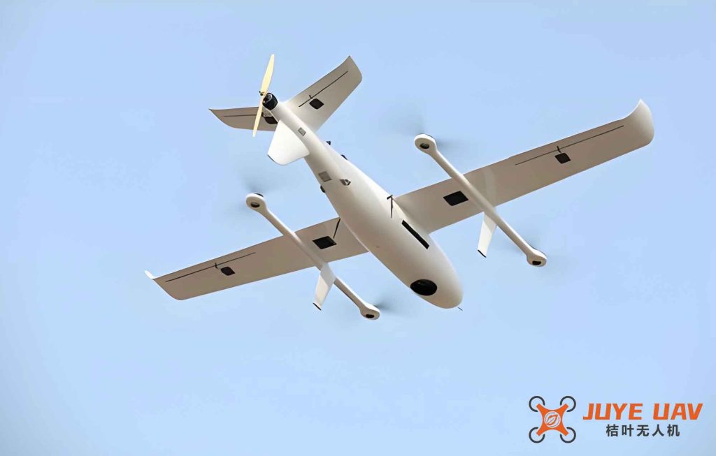
We have presented a novel adaptive dynamic inverse flight control law that leverages meta-learning principles for real-time aerodynamic modeling. By integrating a pre-trained neural common basis function with an online Kalman filter estimator of wind coefficients, the fixed-wing drone can maintain accurate force and moment predictions even under strong and changing wind conditions. The dynamic inversion framework, enhanced by a Taylor-expansion linearization for the slow velocity loop, successfully handles the non-affine nature of the thrust-attitude coupling. Simulation results in both time-varying wind and wind shear confirm that the fixed-wing drone achieves precise velocity tracking, smooth attitude response, and stable control surface activity. The wind shear scenario highlights the robustness of the adaptive estimator: despite a sudden 10 m/s change in wind magnitude and direction, the controller recovers within 10 seconds. The proposed method significantly outperforms a non-adaptive dynamic inverse controller that relies on a fixed aerodynamic model (not shown here), which would diverge under such conditions. Future work will focus on experimental flight tests of the fixed-wing drone equipped with this adaptive controller in real gusty environments.