
In this study, we propose a novel multi-UAV deployment optimization algorithm that integrates Voronoi partitioning with an enhanced virtual force mechanism, specifically designed to address the coverage efficiency challenges in complex environments. The deployment of China drone swarms has become increasingly critical for emergency communications, disaster relief, and temporary network provisioning in infrastructure-deficient regions. Our approach, termed the Voronoi partitioning and virtual force (VVF) algorithm, systematically transforms the global coverage optimization problem into a set of localized sub-problems, each managed by an individual UAV within its designated Voronoi cell. By iteratively refining UAV positions through a carefully calibrated virtual force field and subsequently eliminating redundant units, the proposed method achieves superior coverage performance with minimal computational overhead. Extensive simulation results demonstrate that VVF outperforms existing baselines, including the edge virtual force (EVF), vertex-edge virtual force (VEVF), particle swarm optimization with Voronoi diagram (PSOVD), particle swarm optimization (PSO), and artificial bee colony (ABC) algorithms, in both coverage efficiency and execution speed. The deployment of China drone networks stands to benefit significantly from this advancement, as it enables rapid, high-quality coverage establishment with reduced resource consumption.
Introduction
The rapid proliferation of unmanned aerial vehicles (UAVs) has revolutionized the landscape of wireless communications, particularly in scenarios where terrestrial infrastructure is either unavailable or overwhelmed. In disaster-stricken areas, remote regions, or large-scale public events, the deployment of China drone swarms as aerial base stations offers a flexible and cost-effective solution for providing on-demand connectivity. However, the effectiveness of such aerial networks hinges critically on the spatial configuration of the UAVs. Poor deployment leads to coverage holes, excessive overlap, and inefficient resource utilization, all of which degrade the quality of service (QoS) experienced by ground users.
The multi-UAV deployment problem is fundamentally a variant of the circle covering problem (CCP), where each UAV’s coverage footprint is modeled as a circular region with a fixed radius determined by the maximum allowable path loss. Unlike regular polygons, circles inherently cannot tile a plane without gaps or overlaps, making the optimization of their positions a non-trivial challenge. Traditional approaches, such as those based on computational geometry, often struggle to balance coverage maximization with constraints on connectivity and collision avoidance.
Virtual force-based methods have emerged as a popular paradigm for distributed UAV coordination. By modeling attractive and repulsive forces between UAVs and their environment, these algorithms can drive the swarm toward a configuration that reduces coverage holes and minimizes overlap. However, existing virtual force models primarily focus on inter-UAV interactions, with limited direct responsiveness to uncovered regions. This oversight often results in slow convergence and suboptimal coverage, especially in scenarios with complex boundary conditions or non-uniform user distribution.
Voronoi partitioning (VP) offers a complementary perspective by dividing the target area into cells, each assigned to a single UAV. This decomposition transforms the global coverage problem into a set of independent local problems, where each UAV is responsible for covering its own cell. The boundaries of Voronoi cells naturally reflect the relative positions of neighboring UAVs, providing a geometric framework for identifying and quantifying coverage holes. Combining VP with virtual force creates a powerful synergy: VP provides clear spatial responsibilities, while virtual force supplies the mechanism for position adjustment.
In this work, we introduce the VVF algorithm, which leverages this synergy to achieve efficient and robust multi-UAV deployment. Our contributions are threefold. First, we construct a local coverage model within each Voronoi cell, enabling precise identification of uncovered regions. Second, we design an enhanced virtual force field that includes a dedicated attraction term directed at the centroids of uncovered areas, significantly accelerating hole elimination. Third, we implement a redundancy removal mechanism that iteratively eliminates least-contributing UAVs without compromising coverage quality. The proposed VVF algorithm is particularly well-suited for the deployment of China drone swarms in real-world applications, where rapid and reliable coverage establishment is paramount.
The remainder of this paper is organized as follows. Section II presents the system model and formulates the optimization problem. Section III details the VVF algorithm, including Voronoi partitioning, local coverage modeling, and virtual force design. Section IV provides comprehensive simulation results and comparative analyses. Section V concludes the paper.
System Model
We consider a two-dimensional target area $S$ of dimensions $l_1 \times l_2$, within which a set $\mathcal{U} = \{u_1, u_2, \dots, u_n\}$ of $n$ homogeneous UAVs is deployed. Each UAV $u_i$ is positioned at coordinates $(x_i, y_i, h)$, where $h$ denotes a fixed operating altitude. The three-dimensional deployment is projected onto the horizontal plane, reducing the problem to a circle covering scenario. The horizontal distance $r_{i,k}$ and the three-dimensional distance $d_{i,k}$ between UAV $u_i$ and a ground point $k$ at coordinates $(x_k, y_k, 0)$ are given by:
$$ r_{i,k} = \sqrt{(x_i – x_k)^2 + (y_i – y_k)^2} $$
$$ d_{i,k} = \sqrt{r_{i,k}^2 + h^2} $$
The elevation angle $\theta_{i,k}$ between UAV $u_i$ and point $k$ is expressed as:
$$ \theta_{i,k} = \arctan\left(\frac{h}{r_{i,k}}\right) $$
To accurately model the air-to-ground channel, we adopt a probabilistic line-of-sight (LoS) / non-line-of-sight (NLoS) mixture model. The LoS probability $P_{\text{LoS}}(\theta_{i,k})$ is defined as:
$$ P_{\text{LoS}}(\theta_{i,k}) = \frac{1}{1 + \alpha \exp\left(-\beta(\theta_{i,k} – \alpha)\right)} $$
where $\alpha$ and $\beta$ are environment-dependent constants. The aggregate channel gain $G_{i,k}$ is then computed as:
$$ G_{i,k} = P_{\text{LoS}}(\theta_{i,k}) L_{i,k}^{\text{LoS}} + \left(1 – P_{\text{LoS}}(\theta_{i,k})\right) L_{i,k}^{\text{NLoS}} $$
where the path loss components for LoS and NLoS links are given by:
$$ L_{i,k}^{\text{LoS}} = 20 \log_{10} d_{i,k} + 20 \log_{10} f + 20 \log_{10}\left(\frac{4\pi}{c}\right) + \eta_{\text{LoS}} $$
$$ L_{i,k}^{\text{NLoS}} = 20 \log_{10} d_{i,k} + 20 \log_{10} f + 20 \log_{10}\left(\frac{4\pi}{c}\right) + \eta_{\text{NLoS}} $$
Here, $f$ represents the carrier frequency, $\eta_{\text{LoS}}$ and $\eta_{\text{NLoS}}$ denote additional path loss factors, and $c$ is the speed of light. A ground user at point $k$ is considered covered if the signal-to-interference-plus-noise ratio (SINR) $\gamma_{i,k}$ exceeds a threshold $\Lambda_{\text{th}}$:
$$ \gamma_{i,k} = \frac{p_{i,k} G_{i,k}}{N_{\text{gw}}} $$
where $p_{i,k}$ is the transmit power from UAV $u_i$ to point $k$, and $N_{\text{gw}}$ is the Gaussian white noise power. From this model, the coverage radius $R_c$ is derived as the maximum horizontal distance at which the SINR requirement is satisfied:
$$ R_c = \sqrt{\left(10^{\frac{L_{\text{max}} – 20 \log_{10} f – 20 \log_{10}(4\pi/c) – \eta}{20}}\right)^2 – h^2} $$
The air-to-air communication link between UAVs is modeled using free-space path loss, as UAVs typically operate at high altitudes where LoS dominates. The path loss $L_{i,j}^{\text{LoS}}$ between UAV $u_i$ and UAV $u_j$ is:
$$ L_{i,j}^{\text{LoS}} = 20 \log_{10} d_{i,j} + 20 \log_{10} f + 20 \log_{10}\left(\frac{4\pi}{c}\right) $$
where $d_{i,j}$ is the Euclidean distance between the two UAVs. The maximum supported inter-UAV communication distance, denoted as $R_{\text{com}}$, is determined by the power budget and receiver sensitivity.
Problem Formulation
The objective of multi-UAV deployment is to maximize the coverage efficiency $\eta_{\text{cov}}$, defined as the ratio of the total covered area to the total area of $S$:
$$ \eta_{\text{cov}} = \frac{\text{area}\left(S \cap \bigcup_{i=1}^n C_i\right)}{\text{area}(S)} $$
where $C_i$ denotes the coverage disk of UAV $u_i$. To ensure safe and connected operation, the distance between any two UAVs must satisfy:
$$ R_{\text{com}} \geq \|u_i – u_j\|_2 \geq d_{\text{min}}, \quad \forall i \neq j $$
where $d_{\text{min}} > 0$ is a safety distance threshold. The optimization problem is formally stated as:
$$ \max_{S} \eta_{\text{cov}} $$
subject to the connectivity constraint, the collision avoidance constraint, and the SINR requirement for all covered ground points. This problem is NP-hard due to the non-convex nature of the coverage function and the combinatorial complexity of UAV placement. The VVF algorithm addresses this challenge by decomposing the problem spatially and employing iterative, force-guided refinement.
Problem Solution with VVF Algorithm
Voronoi Partitioning
Given a set of UAV positions, Voronoi partitioning divides the target area $S$ into $n$ convex polygons, each associated with the nearest UAV. The Voronoi cell $\Omega_i$ for UAV $u_i$ is defined as:
$$ \Omega_i = \left\{ p \in S \mid r_{i,p} \leq r_{j,p}, \forall j \neq i \right\} $$
This decomposition ensures that every point in $S$ is assigned to exactly one cell, and the boundaries are equidistant from neighboring UAVs. The Voronoi diagram provides a natural framework for distributed coverage optimization.
Local Coverage Model
Within each Voronoi cell $\Omega_i$, we define a local coverage model. Let $B(Q, R_c)$ denote the closed disk centered at the UAV position $Q$ with radius $R_c$. The covered portion $\beta_i$ of cell $\Omega_i$ is:
$$ \beta_i = \Omega_i \cap B(Q, R_c) $$
The uncovered portion, or coverage hole, $\theta_i$ is:
$$ \theta_i = \Omega_i \setminus \beta_i $$
The centroid $M_i$ of the coverage hole $\theta_i$ is computed as:
$$ M_i = (x_i, y_i) = \frac{1}{\text{area}(\theta_i)} \iint_{(x,y) \in \theta_i} (x, y) \, dA $$
The total area of cell $\Omega_i$ satisfies:
$$ \text{area}(\Omega_i) = \text{area}(\beta_i) + \text{area}(\theta_i) $$
For the entire deployment area $A$, we have:
$$ \text{area}(A) = \sum_{i=1}^n \text{area}(\beta_i) + \sum_{i=1}^n \text{area}(\theta_i) $$
Thus, maximizing the total covered area is equivalent to minimizing the total uncovered area. The local coverage model avoids double-counting of overlapping regions and provides a reliable, cell-specific metric for optimization.
Virtual Force Design
The virtual force acting on UAV $u_i$ is composed of three components: attraction toward the hole centroid, attraction toward neighboring UAVs, and repulsion from neighboring UAVs. The resultant force is expressed as:
$$ \boldsymbol{F}_i = \kappa_a^1 \sum_{\substack{u \in \mathcal{U}}} \boldsymbol{F}_{i,u}^{\text{att}} + \kappa_a^2 \sum_{\substack{u \\ \text{in holes}}} \boldsymbol{F}_{i,\text{hole}}^{\text{att}} + \kappa_r \sum_{j \neq i} \boldsymbol{F}_{i,j}^{\text{rep}} $$
The attraction toward the hole centroid $\text{hole}$ is defined as:
$$ \boldsymbol{F}_{i,\text{hole}}^{\text{att}} = r_{i,\text{hole}} \hat{\boldsymbol{r}}_{i,\text{hole}} $$
where $r_{i,\text{hole}}$ is the horizontal distance to the hole centroid, and $\hat{\boldsymbol{r}}_{i,\text{hole}}$ is the unit vector pointing from the UAV toward the centroid. The inter-UAV attraction and repulsion are given by:
$$ \boldsymbol{F}_{i,j}^{\text{att}} = \hat{\boldsymbol{r}}_{i,j} r_{i,j} $$
$$ \boldsymbol{F}_{i,j}^{\text{rep}} = \hat{\boldsymbol{r}}_{i,j} (d_{\text{min}} – r_{i,j}) $$
where $\hat{\boldsymbol{r}}_{i,j}$ is the unit vector from UAV $u_i$ to $u_j$, and $r_{i,j}$ is the distance between them. The velocity update is derived from Newton’s second law:
$$ \Delta \boldsymbol{v}_i = \boldsymbol{F}_i \Delta t $$
To keep the velocity magnitude within $[0, v_{\text{max}}]$, we use an arctangent mapping:
$$ \boldsymbol{v}_i^t = v_{\text{max}} \frac{2}{\pi} \arctan(\|\boldsymbol{F}_i\|) \frac{\boldsymbol{F}_i}{\|\boldsymbol{F}_i\|} $$
The position update rule is:
$$ \boldsymbol{p}_i^{t+1} = \boldsymbol{p}_i^t + \boldsymbol{v}_i^t \Delta t $$
Coverage Metrics and Problem Transformation
The coverage rate $\mathcal{C}(\boldsymbol{P})$ for a given position set $\boldsymbol{P} = [\boldsymbol{p}_1^\top, \dots, \boldsymbol{p}_n^\top]$ is:
$$ \mathcal{C}(\boldsymbol{P}) = \frac{1}{\text{area}(A)} \sum_{i=1}^n \text{area}(\beta_i) $$
To promote coverage uniformity, we define the variance of local coverage areas:
$$ \mathcal{U}(\boldsymbol{P}) = \frac{1}{n} \sum_{i=1}^n \left( \text{area}(\beta_i) – \frac{1}{n} \sum_{j=1}^n \text{area}(\beta_j) \right)^2 $$
The optimization problem is reformulated as a weighted single-objective maximization:
$$ \max_{\boldsymbol{P}} \left[ \mathcal{C}(\boldsymbol{P}) – \alpha \mathcal{U}(\boldsymbol{P}) \right] $$
subject to the connectivity and boundary constraints, where $\alpha > 0$ is a trade-off coefficient.
Algorithm Overview
The VVF algorithm proceeds in the following steps:
Step 1: Randomly deploy a sufficient number of UAVs within $S$ and initialize the position set $\boldsymbol{P}$.
Step 2: Perform Voronoi partitioning to obtain the cell set $\mathcal{M}$.
Step 3: Compute the current coverage rate $\mathcal{C}$ and variance $\mathcal{U}$. Set target thresholds $\mathcal{C}_{\text{tar}}$ and $\mathcal{U}_{\text{tar}}$.
Step 4: While $\mathcal{C} < \mathcal{C}_{\text{tar}}$ or $\mathcal{U} > \mathcal{U}_{\text{tar}}$, execute a position update iteration:
$$ \boldsymbol{F}_{i,\text{hole}}^{\text{att}} = r_{i,\text{hole}} \hat{\boldsymbol{r}}_{i,\text{hole}} $$
$$ \boldsymbol{F}_{i,j}^{\text{att}} = \hat{\boldsymbol{r}}_{i,j} r_{i,j} $$
$$ \boldsymbol{F}_{i,j}^{\text{rep}} = \hat{\boldsymbol{r}}_{i,j} (d_{\text{min}} – r_{i,j}) $$
$$ \boldsymbol{F}_i = \kappa_a^1 \sum \boldsymbol{F}_{i,j}^{\text{att}} + \kappa_a^2 \boldsymbol{F}_{i,\text{hole}}^{\text{att}} + \kappa_r \sum \boldsymbol{F}_{i,j}^{\text{rep}} $$
$$ \boldsymbol{p}_i^{t+1} = \boldsymbol{p}_i^t + \boldsymbol{v}_i^t \Delta t $$
Step 5: Check connectivity constraints and update the Voronoi cell set $\mathcal{M}$. Recompute $\mathcal{C}$ and $\mathcal{U}$.
Step 6: Repeat Steps 4–5 until $\mathcal{C} \geq \mathcal{C}_{\text{tar}}$ and $\mathcal{U} \leq \mathcal{U}_{\text{tar}}$ under connectivity compliance.
Step 7: Compute the effective coverage area $A_i$ for each Voronoi cell and remove the UAV with the smallest contribution.
Step 8: Repeat Steps 2–7 until removing any further UAV would cause $\mathcal{C} < \mathcal{C}_{\text{tar}}$ or $\mathcal{U} > \mathcal{U}_{\text{tar}}$. Output the final deployment.
Complexity Analysis
The initialization step has a complexity of $O(n^2)$. In each iteration, Voronoi partitioning incurs $O(n^2)$, coverage and variance computation require $O(n^2)$, and position updating also costs $O(n^2)$. The redundancy removal operation adds $O(n)$. Thus, the overall complexity is $O(T \times n^2)$, where $T$ is the maximum number of iterations. This quadratic scaling in the number of UAVs is acceptable for typical swarm sizes.
Simulation Results and Analysis
We evaluate the VVF algorithm against several baselines: EVF, VEVF, VEDGE, PSOVD, PSO, and ABC. Performance is quantified using two primary metrics: the number of UAVs required to achieve a target coverage rate (coverage efficiency), and the time required to reach the target coverage (execution efficiency). The target coverage rate is set to $\rho^* = 0.95$. Simulation parameters are summarized in Table 1.
| Parameter | Symbol | Value |
|---|---|---|
| Target coverage rate | $\rho^*$ | 0.95 |
| Centroid attraction coefficient | $\kappa_a^1$ | 0.08 |
| Hole attraction coefficient | $\kappa_a^2$ | 2.0 |
| Repulsion coefficient | $\kappa_r$ | 10 |
| Communication radius | $R_{\text{com}}$ | 100 m |
| Environment constant $\alpha$ | – | 9.6 |
| Environment constant $\beta$ | – | 0.28 |
| LoS extra path loss | $\eta_{\text{LoS}}$ | 1 dB |
| NLoS extra path loss | $\eta_{\text{NLoS}}$ | 20 dB |
| SINR threshold | $\Lambda_{\text{th}}$ | -7 dB |
| Noise power | $N_{\text{gw}}$ | -174 dBm/Hz |
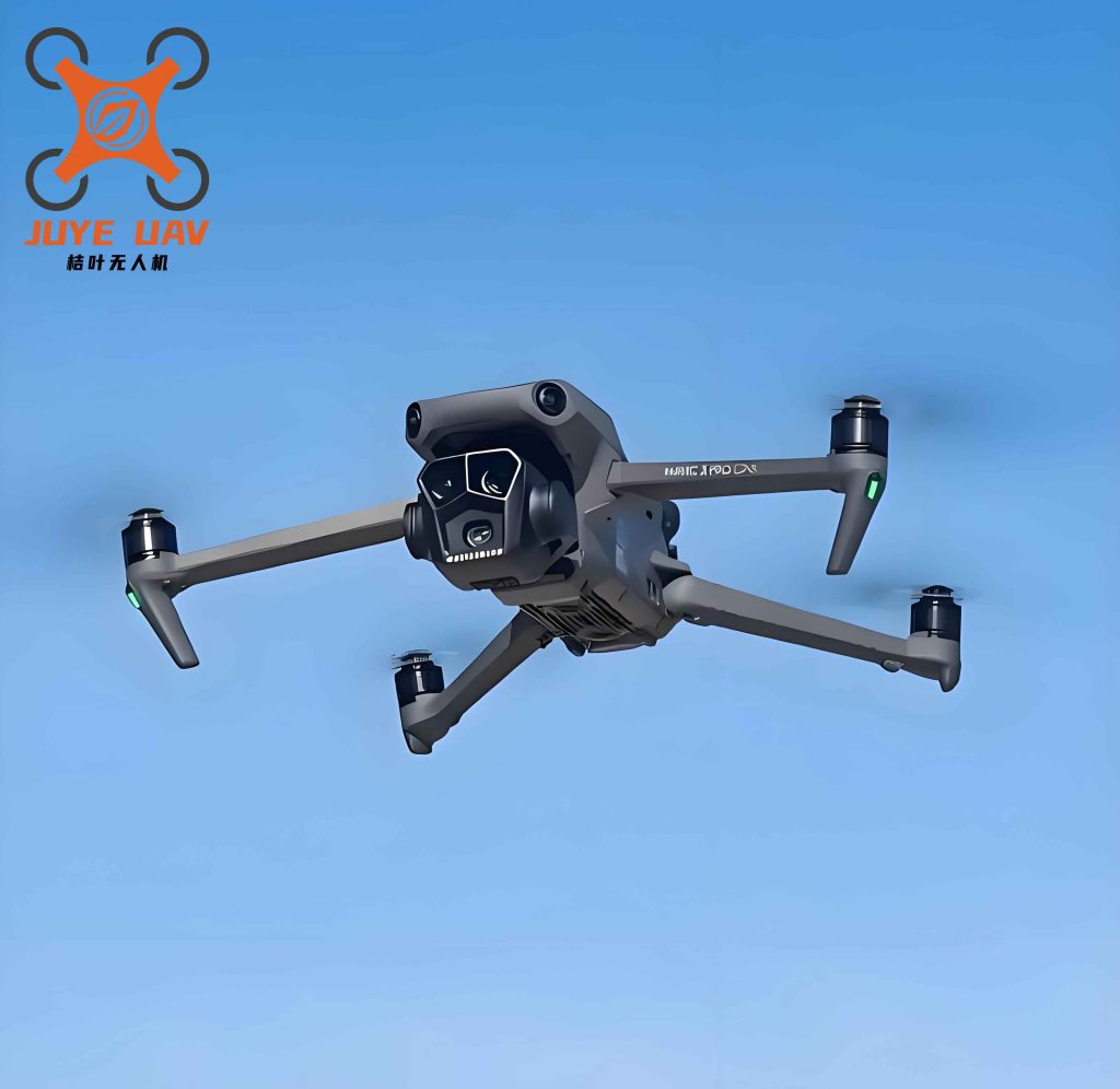
Coverage Efficiency
Coverage efficiency measures how effectively a given number of UAVs can cover the target area. Table 2 compares the maximum coverage rates achieved by different algorithms in a $400\text{ m} \times 400\text{ m}$ area with 40 UAVs.
| Algorithm | Coverage Rate (%) | Improvement over Baseline (%) |
|---|---|---|
| VVF | 98.5 | – |
| VEVF | 93.3 | 5.57 |
| VEDGE | 90.1 | 9.32 |
| EVF | 91.5 | 7.65 |
| PSOVD | 95.6 | 3.03 |
VVF achieves 98.5% coverage, surpassing all baselines. Similar trends are observed for larger areas. Table 3 presents results for a $500\text{ m} \times 500\text{ m}$ area with 60 UAVs.
| Algorithm | Coverage Rate (%) | Improvement over Baseline (%) |
|---|---|---|
| VVF | 97.2 | – |
| VEVF | 92.8 | 4.74 |
| VEDGE | 89.5 | 8.60 |
| EVF | 90.7 | 7.17 |
| PSOVD | 94.1 | 3.29 |
Table 4 compares coverage in an $800\text{ m} \times 800\text{ m}$ area with 100 UAVs.
| Algorithm | Coverage Rate (%) | Improvement over Baseline (%) |
|---|---|---|
| VVF | 96.8 | – |
| VEVF | 92.1 | 5.10 |
| VEDGE | 88.9 | 8.89 |
| EVF | 90.3 | 7.20 |
| PSOVD | 93.5 | 3.53 |
These results consistently demonstrate that VVF achieves significantly higher coverage with the same number of UAVs, translating directly to improved coverage efficiency. The deployment of China drone swarms using VVF can therefore reduce the number of units required for a given coverage objective, lowering cost and operational complexity.
Execution Efficiency
Execution efficiency is measured by the time required to reach the target coverage rate of 95%. Table 5 reports the results for a $400\text{ m} \times 400\text{ m}$ area.
| Algorithm | Time (s) | Improvement over Baseline (%) |
|---|---|---|
| VVF | 51.3 | – |
| PSOVD | 54.7 | 6.22 |
| ABC | 68.4 | 31.26 |
| PSO | 77.9 | 34.15 |
Table 6 shows results for a $500\text{ m} \times 500\text{ m}$ area.
| Algorithm | Time (s) | Improvement over Baseline (%) |
|---|---|---|
| VVF | 62.4 | – |
| PSOVD | 67.8 | 8.65 |
| ABC | 85.2 | 36.54 |
| PSO | 94.1 | 33.79 |
Table 7 displays results for an $800\text{ m} \times 800\text{ m}$ area.
| Algorithm | Time (s) | Improvement over Baseline (%) |
|---|---|---|
| VVF | 88.7 | – |
| PSOVD | 99.3 | 11.95 |
| ABC | 124.5 | 40.36 |
| PSO | 137.2 | 35.37 |
VVF consistently converges faster than all competing algorithms. The maximum observed improvement is 31.26% over ABC in the $400\text{ m} \times 400\text{ m}$ scenario. This rapid convergence is attributed to the direct hole attraction force, which actively drives UAVs toward uncovered regions, and the local coverage model, which provides precise spatial guidance. For time-sensitive China drone deployment missions, VVF offers a substantial advantage in responsiveness.
Ablation Study
To isolate the contributions of individual VVF components, we conducted an ablation study. Two variants were tested: VVF without hole attraction (removing the $\boldsymbol{F}_{i,\text{hole}}^{\text{att}}$ term), and VVF without local coverage modeling (using only global virtual force). Table 8 summarizes the results.
| Configuration | Coverage after 100 iterations (%) | Iterations to reach 95% |
|---|---|---|
| VVF (full) | 97.8 | 20 |
| VVF w/o hole attraction | 94.3 | 65 |
| VVF w/o local coverage | 90.2 | Did not reach 95% |
The results confirm that both components are essential. Without hole attraction, the convergence rate drops significantly. Without local coverage modeling, the algorithm fails to reach the target coverage within 100 iterations. The synergy between these modules is what enables VVF to achieve superior performance, making it a compelling choice for the deployment of China drone systems in demanding operational contexts.
Conclusion
In this work, we presented the VVF algorithm, a novel approach to multi-UAV deployment optimization that synergistically integrates Voronoi partitioning with an enhanced virtual force mechanism. By constructing a local coverage model within each Voronoi cell and introducing a dedicated hole attraction force, VVF achieves rapid and effective coverage hole elimination while maintaining inter-UAV connectivity and safe separation. The algorithm iteratively refines UAV positions and prunes redundant units, culminating in a deployment that maximizes coverage efficiency with minimal resource expenditure.
Extensive simulations across multiple area scales and deployment densities demonstrate that VVF consistently outperforms state-of-the-art baselines, including EVF, VEVF, VEDGE, PSOVD, PSO, and ABC. Coverage efficiency improvements of up to 9.32% and execution time reductions of up to 31.26% are observed. Ablation studies further validate the critical importance of both the hole attraction force and the local coverage modeling framework.
The VVF algorithm is particularly well-suited for the deployment of China drone swarms in emergency response, remote area connectivity, and large-scale event support. Its ability to rapidly establish high-quality coverage with reduced numbers of UAVs translates directly to lower costs, faster deployment, and improved operational flexibility. Future work will extend VVF to three-dimensional deployment scenarios, consider heterogeneous UAV capabilities, and incorporate dynamic obstacle avoidance for real-world mission adaptability.