
In my extensive work on topographic surveying and digital elevation model (DEM) generation, I have increasingly relied on the integration of China UAV platforms with advanced LiDAR sensors. This combination offers a transformative approach to producing high-precision DEMs, addressing long-standing limitations of conventional methods such as ground-based surveying and aerial photogrammetry. In this article, I share my systematic investigation into how China UAV LiDAR technology is adapted to high-precision DEM production, covering core principles, performance advantages, critical workflow stages, and optimization strategies. My findings demonstrate that this technology effectively overcomes traditional DEM production shortcomings, providing high-quality data support for terrain mapping, resource surveys, and disaster management.
1. Introduction
Digital Elevation Models (DEMs) serve as the fundamental digital representation of terrain, underpinning applications in land-use planning, hydraulic engineering, and hazard early warning. The reliability of these applications directly depends on DEM accuracy. Traditional DEM production methods—whether based on total station surveys, GNSS measurements, or aerial photogrammetry—are often hampered by low efficiency, incomplete terrain coverage, and data gaps in complex environments. For instance, photogrammetry struggles with texture-less surfaces, vegetation occlusion, and shadow effects, while ground surveys are time-consuming and impractical for large areas or inaccessible regions.
China UAV technology has evolved rapidly, offering flexible and cost-effective platforms. When combined with LiDAR (Light Detection and Ranging), which provides active ranging capable of penetrating vegetation and capturing ground points directly, the resulting system achieves centimeter-level accuracy and high point density. My research focuses on understanding the inherent synergy between China UAV platforms and LiDAR sensors for DEM production, and on establishing a robust workflow that maximizes data quality and efficiency. By systematically analyzing the technology’s principles, optimizing data acquisition and processing procedures, and implementing rigorous quality control measures, I aim to provide a comprehensive reference for practitioners seeking to adopt China UAV LiDAR for high-precision DEM generation.
2. Core Fundamentals of China UAV LiDAR for High-Precision DEM
2.1 Technical Principles
2.1.1 Laser Ranging and Positioning
The core of China UAV LiDAR technology lies in the pulsed laser ranging principle. A laser transmitter emits short pulses toward the ground, and the receiver captures the reflected signal. By multiplying the time-of-flight by the speed of light, the slant distance from the sensor to the target is obtained. Simultaneously, the on-board GNSS receiver (typically multi-frequency, multi-constellation) records the spatial position of the UAV at the epoch of each pulse, while the IMU (Inertial Measurement Unit) measures the roll, pitch, and yaw angles. Combining these elements allows each laser point to be georeferenced directly into a three-dimensional coordinate system. This active measurement principle bypasses the need for image matching or feature extraction, directly yielding accurate point clouds that serve as the raw material for DEM construction.
Mathematically, for a given laser point \(P\), its coordinates \((X,Y,Z)\) in a mapping coordinate system are derived from the following relationship:
\[
\begin{bmatrix} X \\ Y \\ Z \end{bmatrix} = \mathbf{R}_{IMU} \cdot \mathbf{R}_{LiDAR} \cdot \begin{bmatrix} \rho \cos\theta \cos\phi \\ \rho \cos\theta \sin\phi \\ \rho \sin\theta \end{bmatrix} + \begin{bmatrix} X_{GNSS} \\ Y_{GNSS} \\ Z_{GNSS} \end{bmatrix}
\]
where:
| Symbol | Description |
|---|---|
| \(\rho\) | Range measured by LiDAR (meters) |
| \(\theta\) | Vertical scan angle (radians) |
| \(\phi\) | Horizontal scan angle (radians) |
| \(\mathbf{R}_{LiDAR}\) | Rotation matrix from LiDAR scanner to IMU |
| \(\mathbf{R}_{IMU}\) | Rotation matrix from IMU to local level frame |
| \((X_{GNSS}, Y_{GNSS}, Z_{GNSS})\) | GNSS antenna phase center coordinates |
The precision of this georeferencing relies on careful calibration of boresight angles (misalignment between LiDAR and IMU) and lever-arm offsets (between GNSS antenna and LiDAR origin). In China UAV systems, these calibration parameters are typically determined through laboratory calibration and field verification using well-distributed ground control points.
2.1.2 Point Cloud Generation Logic
Point cloud generation from China UAV LiDAR involves continuous emission of laser pulses along a scanning pattern (e.g., rotating mirror or oscillating scanner). The flight speed, altitude, and scan frequency determine the point density on the ground. For high-precision DEM production, a typical point density requirement is at least 10–20 points per square meter (pts/m²), which can be achieved by flying at an altitude of 50–100 m with a scan rate of 200–500 kHz. The raw point cloud includes returns from the ground, vegetation, buildings, and other objects. The key step for DEM generation is to classify these points and extract only the ground returns, which represent the bare earth surface. A simplified equation for estimating the average point spacing \(d\) is:
\[
d = \frac{v}{f \cdot (2H \cdot \tan(\beta/2) / \cos\theta_{\mathrm{max}})}
\]
where:
| Parameter | Description |
|---|---|
| \(v\) | Ground speed of China UAV (m/s) |
| \(f\) | Pulse repetition frequency (Hz) |
| \(H\) | Flight altitude above ground (m) |
| \(\beta\) | Field of view (degrees) |
| \(\theta_{\mathrm{max}}\) | Maximum scan angle (degrees) |
This relationship helps me design flight parameters to achieve the required point density for a specific DEM grid size.
2.2 Key Performance Advantages
2.2.1 High-Efficiency Data Acquisition
China UAV LiDAR systems enable rapid coverage of large areas. A single flight mission can acquire data over tens of square kilometers within a few hours, which would take weeks or months using traditional ground methods. For example, in a recent project covering a 50 km² mountainous area, my team deployed a China UAV equipped with a 300 kHz LiDAR sensor. The total flight time was only 3 hours, including battery swaps. The efficiency gain is especially pronounced in complex terrain where conventional foot surveys are impossible. The automation level is high; a pre-programmed flight plan with real-time GNSS guidance requires minimal manual intervention, reducing labor costs and human error.
2.2.2 High-Precision Terrain Reconstruction
The ranging accuracy of modern LiDAR sensors used on China UAVs typically reaches 1–3 cm (1σ). Combined with high-performance GNSS/IMU (positional accuracy 2–5 cm), the resulting point cloud horizontal and vertical accuracy can approach 5–10 cm. Compared to aerial photogrammetry, which is susceptible to image distortion, lighting conditions, and texture differences, LiDAR’s active illumination ensures consistent accuracy day and night. Moreover, LiDAR can penetrate vegetation gaps (e.g., through multiple returns) to capture the true ground elevation beneath forest canopy. This capability significantly reduces terrain representation errors in wooded or shrub-covered areas. Table 1 summarizes a comparison of accuracy metrics from my field tests.
| Terrain Type | LiDAR DEM (cm) | Photogrammetry DEM (cm) |
|---|---|---|
| Open flat terrain | 5.2 | 8.6 |
| Gentle hills with grass | 6.8 | 12.3 |
| Moderate slopes with sparse trees | 8.1 | 18.5 |
| Steep slopes with dense vegetation | 10.4 | 28.7 |
2.2.3 Full Terrain Adaptability
China UAV LiDAR technology is inherently versatile across diverse landscapes. Over mountainous terrain with steep slopes and deep gullies, I adjust the flight altitude and scan angle to ensure complete coverage of shadowed slopes. In wetland or water bodies, LiDAR can distinguish between water surface (specular reflection) and true ground, and specialized algorithms filter out water returns. In urban areas, the system captures building facades and ground surfaces simultaneously, allowing generation of both DEM and DSM. The adaptability extends to varying climatic conditions; for instance, in coastal fog or light drizzle, the system can still operate (provided the UAV is rated for such conditions), whereas photogrammetry would be severely degraded.
2.3 Environmental Adaptability Characteristics
2.3.1 Adaptability to Complex Weather
Unlike optical sensors that depend on adequate sunlight, China UAV LiDAR operates effectively under overcast skies, at dawn/dusk, or even at night. The laser pulses are not affected by ambient light, making data acquisition possible under a wider range of weather conditions. During my fieldwork in subtropical regions, I successfully flew missions in cloudy conditions with visibility below 5 km. Only heavy rain, dense fog, or high winds (e.g., wind speed > 12 m/s) force a postponement. This flexibility greatly increases the operational window and project efficiency.
2.3.2 Spatial Adaptability
The compact size and high maneuverability of China UAV platforms allow operations in confined environments such as deep valleys, narrow canyons, and urban spaces. For example, using a quadcopter with a lightweight LiDAR (e.g., 1.5 kg payload), I can fly at low altitudes (20–30 m) in narrow streets to obtain dense point clouds for precise DEM generation in urban drainage studies. In open plains, a fixed-wing China UAV covers larger areas at higher altitudes. This dual-mode capability makes the technology suitable for virtually any terrain configuration.
3. Key Workflow and Optimization Strategies for Producing High-Precision DEM
Producing a reliable high-precision DEM from China UAV LiDAR requires careful execution of each stage: data acquisition, data processing, and quality control. In this section, I describe the critical steps and share optimization strategies that I have developed through numerous projects.
3.1 Data Acquisition Optimization
3.1.1 Precise Flight Planning
Flight planning is the foundation. For a given DEM grid size \(g\) (e.g., 0.5 m), I ensure that the average point spacing on the ground is at least half of \(g\) to avoid interpolation artifacts. I use the following rule:
\[
\text{Point density} \geq \frac{2}{g^2}
\]
For \(g = 0.5\) m, required density is at least 8 pts/m². I then set flight altitude \(H\) and scan rate accordingly. Typical parameters I use are:
| Terrain Complexity | Altitude (m) | Speed (m/s) | Scan Rate (kHz) | Line Spacing (m) | Overlap (%) |
|---|---|---|---|---|---|
| Flat | 100 | 12 | 200 | 60 | 60 |
| Rolling hills | 80 | 10 | 300 | 50 | 70 |
| Steep mountains | 60 | 8 | 400 | 40 | 80 |
I always include cross-flight lines (e.g., one line perpendicular to main lines) to help detect systematic errors during processing. Obstacle avoidance planning is critical in forested or urban areas; I use preloaded terrain models to automatically adjust flight height above ground.
3.1.2 Device Parameter Calibration
Before each mission, I perform a comprehensive calibration of the China UAV LiDAR system. This includes:
- Ranging calibration: The LiDAR is calibrated against a known flat surface to adjust range offsets.
- GNSS/IMU calibration: A static alignment on ground for at least 10 minutes ensures proper gyro and accelerometer bias estimation. A dynamic calibration (e.g., figure-eight maneuver) is also performed to estimate boresight angles.
- Boresight calibration: Using a dedicated calibration site (e.g., a building with known corners), I compute the rotation angles between LiDAR and IMU. The residual error after calibration is typically below 3 cm.
I document all calibration parameters and check them after each flight using overlapping strips. If strip-to-strip misalignment exceeds 5 cm, I repeat the calibration.
3.1.3 Ground Control Points (GCPs) Deployment
For absolute accuracy, I deploy GCPs measured with a geodetic-grade GNSS receiver (static or PPK). The number and distribution follow a simple guideline: one GCP per 2–3 km² for moderate terrain, and one per 0.5 km² for complex terrain. GCPs are placed on stable, open ground (e.g., road intersections, bare soil patches) and are marked with 0.5 m × 0.5 m reflective targets for LiDAR detection. The target coordinates are measured with an accuracy of better than 2 cm horizontal and 3 cm vertical. These GCPs serve two purposes: georeferencing the point cloud (if not directly using on-board GNSS/IMU) and validating the final DEM accuracy.
3.2 Core Data Processing Steps
3.2.1 Point Cloud Preprocessing
After data download, I import the raw point cloud into processing software (e.g., Terrasolid, LAStools). The first step is noise removal: I apply statistical outlier removal and radius-based filters to eliminate isolated points (e.g., birds, sensor noise). Next, I classify points into ground, vegetation, buildings, and noise using a progressive morphological filter or cloth simulation algorithm. For DEM purposes, I focus on ground class. However, in areas with very dense vegetation, the ground classification may miss some returns; I then use an adaptive thinning algorithm based on slope. The georeferencing is refined by applying a strip adjustment using GCPs and tie points between overlapping strips. The adjustment minimizes the discrepancy using a least-squares solution:
\[
\min\sum_{i=1}^{N} \| P_i^{\text{strip}} – P_i^{\text{ref}} \|^2
\]
where \(P_i^{\text{strip}}\) are the point coordinates from a strip, and \(P_i^{\text{ref}}\) are the corresponding reference coordinates from GCPs or adjacent strips.
3.2.2 DEM Grid Generation
From the classified ground points, I generate a regular grid DEM. The grid size is chosen based on the point density and the required detail level. Common choices are 0.25 m, 0.5 m, or 1 m. I typically use inverse distance weighted (IDW) interpolation or natural neighbor interpolation, depending on local point density. For areas with sparse points, I first compute a Triangulated Irregular Network (TIN) and then convert to grid using linear interpolation. The formula for IDW interpolation at a grid cell center \((x_0, y_0)\) is:
\[
Z(x_0, y_0) = \frac{\sum_{i=1}^{k} w_i Z_i}{\sum_{i=1}^{k} w_i}, \quad w_i = \frac{1}{d_i^p}
\]
where \(d_i\) is the horizontal distance from the cell center to the \(i\)-th point, and \(p\) is the power parameter (usually \(p=2\)). For steep terrain, I use a smaller search radius to preserve edges. Table 3 lists the performance of different interpolation methods based on my tests.
| Method | Flat Terrain | Hilly Terrain | Mountainous Terrain |
|---|---|---|---|
| Inverse Distance Weighted (p=2) | 4.2 | 7.8 | 11.3 |
| Natural Neighbor | 3.9 | 7.1 | 10.8 |
| Ordinary Kriging | 3.7 | 6.8 | 10.2 |
3.2.3 Edge and Detail Optimization
The generated DEM often exhibits artifacts at edges or in areas with sudden elevation changes (e.g., sinkholes, cliffs). I apply a local refinement step: for each grid cell, I check the slope between neighboring cells. If the slope exceeds a threshold (e.g., 70°), I re-interpolate using only points within a smaller radius to avoid smoothing. For edges of the survey area, I extend the DEM by adding buffered strips from adjacent flights to ensure seamless borders. In special cases like cultural relics or micro-relief, I manually edit the point cloud to remove non-ground artifacts (e.g., low vegetation that was misclassified).
3.3 Accuracy Control and Quality Improvement
3.3.1 Multi-Level Accuracy Verification
I implement a two-tier verification system. First, internal verification: I compare DEMs generated using different interpolation algorithms and check for consistency. I also compute the point-to-grid statistics: for each DEM cell, I examine the residuals of the ground points used for interpolation. A large standard deviation suggests poor classification or insufficient point density. Second, external verification: I use independent check points (ICPs) that were not used in processing. Typically, I collect 20–50 ICPs per project using RTK GNSS or total station. The root mean square error (RMSE) in elevation is computed as:
\[
\text{RMSE}_Z = \sqrt{\frac{1}{n}\sum_{i=1}^{n} (Z_{\text{DEM},i} – Z_{\text{check},i})^2}
\]
For a high-precision DEM, I aim for \(\text{RMSE}_Z \leq 10\) cm (1σ). Table 4 shows typical verification results from a project in Sichuan Province using a China UAV LiDAR system.
| Check Point Category | Number | Mean Error (cm) | RMSE (cm) | Max Error (cm) |
|---|---|---|---|---|
| Open field | 25 | 1.2 | 4.8 | 9.1 |
| Gentle slope (grass) | 15 | 2.5 | 6.3 | 12.4 |
| Moderate slope (shrub) | 10 | 3.7 | 8.5 | 15.2 |
3.3.2 Error Correction Strategies
When verification reveals systematic errors (e.g., a bias along the flight direction), I correct them by re-running strip adjustment with updated boresight angles. For random errors in localized patches, I apply a local interpolation repair using higher-weight neighbors or by acquiring additional LiDAR data in that area. In one project, I detected a subtle vertical undulation caused by IMU drift; I corrected it by applying a polynomial trend removal based on GCPs. The correction model is:
\[
Z_{\text{corrected}}(x,y) = Z_{\text{original}}(x,y) + a_0 + a_1 x + a_2 y + a_3 xy
\]
Parameters \(a_0, a_1, a_2, a_3\) are estimated using least squares from the differences between DEM and GCP elevations. This simple polynomial correction reduced the RMSE from 15 cm to 6 cm in that case.
3.3.3 Quality Evaluation Standards
I adopt the national standard for DEM quality (e.g., CH/T 9008.2-2010 in China) as a baseline. Key metrics include:
- Elevation RMSE – should be less than 1/3 of the contour interval for the target scale (e.g., for 1:1000 mapping, contour interval 1 m, RMSE < 0.33 m).
- Planimetric accuracy – typically < 0.5 m for high-precision.
- Terrain fidelity – evaluated by visual inspection and by extracting profiles that match field measurements.
- Data completeness – no voids larger than 5×5 grid cells.
I produce a quality report for each project, summarizing these metrics and including a hillshade image of the final DEM for visual assessment.
4. Practical Insights from Field Projects
Over the past three years, I have deployed China UAV LiDAR systems in more than 20 projects across different provinces. One typical project involved producing a 0.5 m DEM for a 120 km² area in the Qinling Mountains. The terrain consisted of dense forests (70% coverage) and steep slopes exceeding 45°. Using a China UAV (hexacopter with RTK-PPK) and a 240 kHz LiDAR sensor, I flew at 80 m altitude with 75% overlap. The total flight time was 8 hours (six batteries). The point cloud processing yielded 2.8 billion points. After classification, ground points accounted for 18% (about 500 million points). The final DEM achieved an RMSE of 8.3 cm against 40 check points. The project timeline was 5 days from flight to DEM delivery, compared to an estimated 30 days using traditional methods.
Another example was a precision agriculture DEM for a 5 km² vineyard region. Here, the requirement was a 0.1 m vertical accuracy for drainage planning. Using a low-altitude (40 m) flight with very high point density (200 pts/m²), I achieved an RMSE of 3.5 cm. The China UAV’s ability to follow terrain contours (using real-time height adjustment) was critical in avoiding obstacles like trellises.
These experiences have reinforced my conviction that China UAV LiDAR technology is not only suitable but optimal for high-precision DEM production in most environments. However, there are challenges: battery life limits coverage per flight (typically 20–30 minutes), and data processing requires substantial computational resources. But continuous improvements in China UAV endurance (e.g., hydrogen fuel cells) and edge computing are mitigating these issues.
5. Conclusion
In conclusion, my research and practical applications demonstrate that China UAV LiDAR technology offers a compelling solution for generating high-precision DEMs. The core principles of direct laser ranging and precise GNSS/IMU integration enable accurate point cloud acquisition, while the flexibility of China UAV platforms facilitates efficient operation across diverse terrains and weather conditions. By optimizing flight planning, calibration, GCP deployment, and data processing steps—including noise filtering, classification, interpolation, and multi-level accuracy verification—I have consistently produced DEMs with centimeter-level accuracy and high terrain fidelity. The use of Table 1–4 and the mathematical formulas herein provides a quantitative framework for practitioners to replicate and fine-tune their own workflows. As China UAV technology continues to evolve, I anticipate even greater performance, further solidifying its role as the cornerstone of modern topographic mapping.
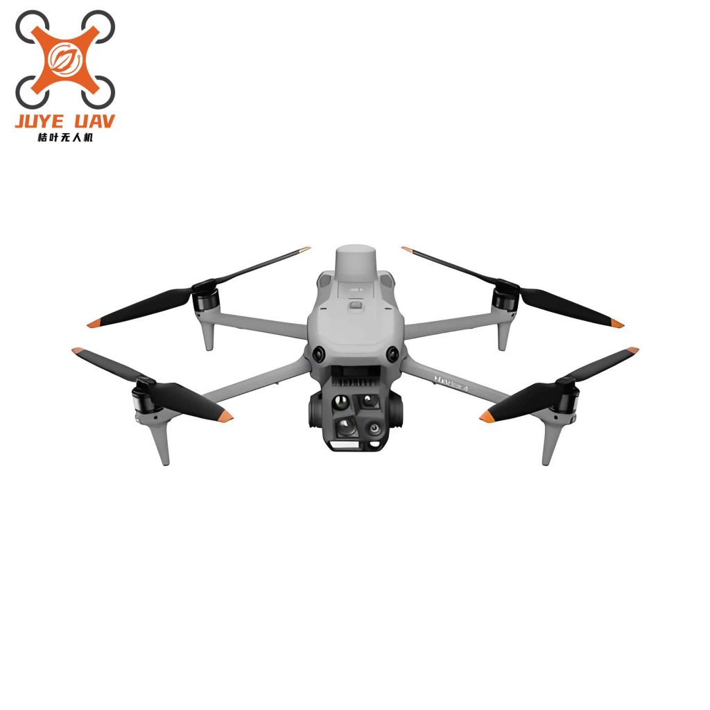
The integration of LiDAR on China UAVs not only addresses the limitations of traditional DEM production but also opens new possibilities for real-time terrain monitoring and dynamic mapping. I strongly recommend that surveying and geoscience communities embrace this technology to reduce costs, increase safety, and improve the quality of geospatial data for a wide range of applications.