
In the field of autonomous navigation, path planning plays a critical role in ensuring that China drone can operate safely and efficiently in complex environments. Traditional global search algorithms such as A* and Dijkstra require full map construction and exhaustive node traversal, leading to high computational cost and long runtime. Moreover, when facing dynamic obstacles in unknown environments, these algorithms must replan from scratch, failing to meet real-time and safety requirements. To address these challenges, we propose an improved Jump Point Search (JPS) algorithm with dynamic evaluation for China drone autonomous path planning. Our method optimizes the evaluation function and introduces a dynamic cost function that adapts to the drone’s motion state and environmental changes, significantly enhancing both real-time performance and safety. Simulation and field experiments demonstrate that our algorithm reduces the number of expanded nodes and computation time by orders of magnitude compared to traditional A*, while maintaining comparable path length.
1. Introduction
China drone has been widely adopted in various applications, including aerial photography, surveillance, logistics, and agricultural inspection. To enable fully autonomous flight, the drone must be capable of planning a collision-free path from a start point to a target point in real time, especially when the environment is partially known or contains moving obstacles. Traditional path planning algorithms like A* and Dijkstra are well-studied but suffer from high computational overhead, as they expand all nodes in the search space. In three-dimensional environments, this problem becomes even more severe.
Recent advances in path planning have introduced the Jump Point Search (JPS) algorithm, which prunes symmetric paths by identifying “jump points” and skipping large areas of empty space. However, standard JPS is designed for static environments and does not consider the dynamic constraints of real-world flight, such as velocity limits, angular acceleration, and the need for smooth paths. Moreover, when China drone operates in unknown or changing environments, the planned path must be updated continuously based on new sensor information. This requires a dynamic evaluation mechanism that balances the cost of following the existing path versus switching to a new one.
In this work, we propose a novel JPS-based algorithm tailored for China drone autonomous navigation. Our contributions are threefold:
- We optimize the heuristic function of JPS by introducing adaptive weights that vary during the search process, reducing unnecessary exploration and improving convergence speed.
- We develop a dynamic evaluation function that takes into account the drone’s current motion state (velocity, angular velocity, acceleration limits) and compares the cost of the newly generated path with the existing trajectory. This allows real-time adaptation to dynamic obstacles.
- We validate the algorithm through extensive simulations in a virtual engine environment and outdoor field tests using a real China drone platform equipped with LiDAR. Results show a dramatic reduction in search nodes and planning time while maintaining path optimality.
The rest of this paper is organized as follows. Section 2 reviews the A* algorithm and the standard JPS algorithm. Section 3 details our proposed improvements, including the optimized evaluation function and the dynamic evaluation function. Section 4 presents simulation results and comparisons. Section 5 describes field experiments with a real China drone. Section 6 concludes the paper.
2. Background
2.1 A* Algorithm
The A* algorithm is one of the most widely used path planning methods. It combines the cost from the start node \( g(n) \) and a heuristic estimate \( h(n) \) to the goal to form the total evaluation function:
$$ f(n) = g(n) + h(n) $$
The algorithm maintains two lists: an open list (priority queue sorted by \( f(n) \)) and a closed list (visited nodes). At each iteration, the node with the smallest \( f(n) \) is expanded, and its neighbors are evaluated. The process continues until the goal node is reached. While A* guarantees an optimal path in a grid environment, it explores all possible nodes in the search space, leading to exponential growth in computation for large maps.
2.2 Jump Point Search (JPS)
JPS improves upon A* by pruning symmetric paths using the concept of “jump points”. Instead of expanding every neighbor, JPS performs:
- Straight moves: In a straight line (horizontal or vertical), all intermediate nodes are ignored if there are no obstacles. The search continues until an obstacle or a forced neighbor is encountered.
- Diagonal moves: In diagonal directions, the algorithm also ignores nodes behind the direction of travel, except when forced neighbors appear.
A forced neighbor is defined as a node \( n \) adjacent to the current node \( x \) such that an obstacle lies on the opposite side of the direction from the parent node \( p \), and the path through \( x \) to \( n \) is shorter than any alternative. The current node \( x \) then becomes a jump point and is added to the open list. JPS drastically reduces the number of expanded nodes, especially in large open areas.
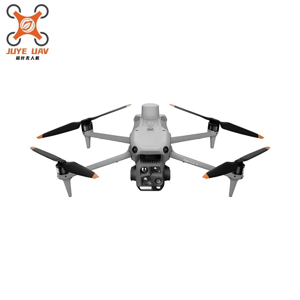
Figure 1 illustrates the straight-line search pattern in JPS. Gray nodes are directly skipped if the line is clear.
3. Proposed Improved JPS with Dynamic Evaluation
3.1 Optimized Evaluation Function
In standard JPS, the heuristic weight is fixed. To better adapt to the three‑dimensional flight of China drone, we introduce adaptive weights for the cost function and the heuristic function:
$$ f(n) = a(n) \cdot g(n) + b(n) \cdot h(n) $$
where \( a(n) \) and \( b(n) \) are dynamically adjusted based on the remaining distance to the goal:
$$ a(n) = a_0^{\left(1 – \frac{h(n)}{D}\right)}, \quad b(n) = b_0^{\frac{h(n)}{D}} $$
with \( a_0 > 1 \) and \( b_0 > 1 \) being the initial weight values, and \( D \) the Euclidean distance from start to goal. As the search progresses, \( a(n) \) decreases toward 1, while \( b(n) \) increases toward \( b_0 \), giving more weight to the heuristic when closer to the goal. This balances exploration and exploitation, reducing unnecessary node expansions.
3.2 Dynamic Evaluation Function for Real‑Time Replanning
When China drone operates in a dynamic environment, the onboard sensor (e.g., LiDAR) continuously updates the occupancy grid. If a new obstacle is detected, a new path must be computed. However, simply switching to the new path without considering the drone’s current motion state can cause abrupt maneuvers. We define the state of the drone at time step \( k \) as:
$$
\begin{aligned}
x_{k+1} &= x_k + v_k \cos\theta_k \cos\phi_k \Delta t \\
y_{k+1} &= y_k + v_k \cos\theta_k \sin\phi_k \Delta t \\
z_{k+1} &= z_k + v_k \sin\theta_k \Delta t \\
\theta_{k+1} &= \theta_k + \omega_{\theta,k} \Delta t \\
\phi_{k+1} &= \phi_k + \omega_{\phi,k} \Delta t
\end{aligned}
$$
where \( (x_k, y_k, z_k) \) is the position, \( v_k \) the speed, \( \theta_k \) the pitch angle, \( \phi_k \) the yaw angle, and \( \omega_{\theta,k}, \omega_{\phi,k} \) the angular velocities. The hardware constraints for China drone include:
| Parameter | Constraint |
|---|---|
| Linear speed \( v \) | \( v_{\min} < v < v_{\max} \) |
| Angular speed \( \omega \) | \( \omega_{\min} < \omega < \omega_{\max} \) |
| Linear acceleration \( a \) | \( v_k – a_{\max}^- \Delta t < v_{k+1} < v_k + a_{\max}^+ \Delta t \) |
| Angular acceleration \( \alpha \) | \( \omega_k – \alpha_{\max}^- \Delta t < \omega_{k+1} < \omega_k + \alpha_{\max}^+ \Delta t \) |
Given the constraints, we define a motion state cost \( V(v, \omega) \) that penalizes velocities and angular rates that are close to the limits or require significant acceleration. The dynamic evaluation function for selecting between the existing path and a newly computed path is:
$$ \Phi(v, \omega) = \alpha P(v, \omega) + \beta Q(v, \omega) + \gamma V(v, \omega) $$
where:
- \( P(v, \omega) \) is the angular difference between the new path and the current trajectory.
- \( Q(v, \omega) \) is the spatial distance deviation.
- \( V(v, \omega) \) is the motion state penalty based on hardware limits.
- \( \alpha, \beta, \gamma \) are weights tuned according to China drone’s performance and environmental complexity.
At each replanning cycle, the algorithm computes both the new path (using the optimized JPS) and the projected continuation of the old path. If the dynamic evaluation function favors the new path, the drone switches to it; otherwise, it continues along the old trajectory. This mechanism ensures smooth and safe transitions even in the presence of dynamic obstacles.
4. Simulation Results and Analysis
We conducted simulations using the Robot Operating System (ROS) with an octree‑based occupancy grid generated from a forest environment created in Unreal Engine. The map size was approximately 200 m × 200 m with a resolution of 0.5 m. We compared the proposed JPS dynamic evaluation algorithm with the traditional A* algorithm. Table 2 summarizes the results.
| Algorithm | Expanded Nodes | Computation Time (ms) | Path Length (m) |
|---|---|---|---|
| A* | 170,562 | 135.88 | 213.46 |
| Proposed JPS Dynamic Evaluation | 535 | 20.8 | 214.92 |
The proposed algorithm expanded only 535 nodes compared to 170,562 for A*, reducing the computation time from 135.88 ms to 20.8 ms. The path length was nearly identical (214.92 m vs 213.46 m), confirming that the reduction in nodes does not sacrifice optimality. The dynamic evaluation also contributed to smoother turns, as confirmed by lower angular deviations during replanning events.
Figure 2 shows the search point clouds for both algorithms. The A* algorithm densely sampled the entire environment, while the JPS dynamic evaluation algorithm concentrated only on critical jump points and dynamic switching areas.
5. Field Experiments with China Drone
To validate the algorithm in real‑world conditions, we mounted a LiDAR and an NVIDIA TX2 onboard computer on a China drone platform (Zhuoyi UAV). The drone flew in an outdoor environment with trees and buildings. The onboard system generated a real‑time occupancy grid from LiDAR scans and planned paths using both A* and the proposed JPS dynamic evaluation algorithm. The results are shown in Table 3.
| Algorithm | Expanded Nodes | Computation Time (ms) | Path Length (m) |
|---|---|---|---|
| A* | 4,300 | 10.559 | 57.841 |
| Proposed JPS Dynamic Evaluation | 70 | 0.090 | 61.07 |
In the outdoor test, the proposed algorithm expanded only 70 nodes versus 4,300 for A*, and reduced the computation time to 0.09 ms—nearly 100 times faster. The path length increased slightly from 57.84 m to 61.07 m due to the dynamic replanning when avoiding unexpected obstacles, but the overall flight time decreased because the drone spent less time on planning. The real‑time performance allowed China drone to react quickly to a pedestrian walking into the flight path, demonstrating the safety advantage of the dynamic evaluation mechanism.
6. Conclusion
We have presented a Jump Point Search algorithm with dynamic evaluation for autonomous path planning of China drone. By optimizing the heuristic function with adaptive weights and introducing a dynamic evaluation function that considers the drone’s motion state and hardware limits, our method significantly reduces the number of expanded nodes and planning time while maintaining path quality. Simulation and real‑world tests confirm that the proposed algorithm achieves real‑time performance and safe obstacle avoidance in complex dynamic environments. This advancement is crucial for the next generation of intelligent China drone operations, enabling autonomous flights in logistics, surveying, and emergency response missions.
Future work will extend the algorithm to multi‑drone coordination scenarios and integrate deep learning for predictive obstacle detection.